Last modified: Jan 31 2026 at 10:09 PM • 11 mins read

Why Deep Representations?

Introduction
Intuition 1: Hierarchical Feature Learning
Connection to Neuroscience
Intuition 2: Circuit Theory
Practical Considerations
Summary: Why Depth Matters
Key Takeaways

Introduction

Deep neural networks consistently outperform shallow networks across many applications. But why does depth matter so much? It’s not just about having more parameters—there’s something special about having many layers.

In this lesson, we’ll explore:

Hierarchical feature learning: How deep networks build complex features from simple ones
Circuit theory perspective: Mathematical reasons for preferring depth
Practical insights: When and why to use deep architectures

Key Question: Why can’t we just use a shallow network with more hidden units instead of a deep network?

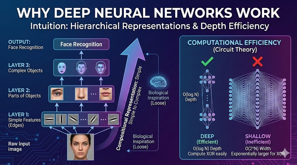
Intuition 1: Hierarchical Feature Learning

Example: Face Recognition

Let’s understand what a deep neural network computes when performing face recognition or detection.

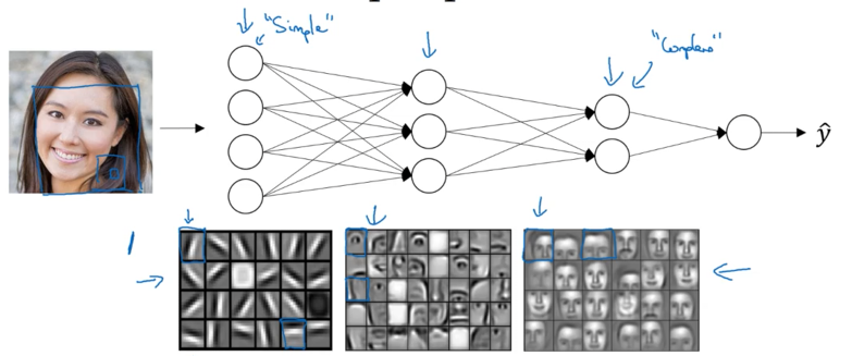
Layer-by-Layer Feature Hierarchy

Layer 1: Edge Detection

The first layer acts as an edge detector:

Input: Raw image pixels (face photo)
         ↓
Layer 1: Detect edges (20 hidden units)
         • Vertical edges: |
         • Horizontal edges: —
         • Diagonal edges: / \
         • Various orientations

Each hidden unit learns to detect edges at different orientations in small regions of the image.

Note: When we study convolutional neural networks in a later course, this visualization will make even more sense!

How it works:

First layer groups pixels → edges
Looks at small local regions of the image
Each hidden unit specializes in one edge orientation

Layer 2: Facial Parts Detection

The second layer combines edges to detect facial parts:

Edges (from Layer 1)
         ↓
Layer 2: Detect facial parts
         • Eyes
         • Nose
         • Mouth
         • Ears
         • Eyebrows

By combining multiple edges, the network learns to recognize meaningful parts of a face.

Layer 3 & 4: Complete Face Recognition

Deeper layers combine facial parts to recognize complete faces:

Facial parts (from Layer 2)
         ↓
Layer 3 & 4: Detect faces
         • Different face shapes
         • Various expressions
         • Different people
         • Face orientations

By composing eyes, nose, ears, and chin together, the network recognizes complete faces and identifies individuals.

The Hierarchical Pattern

Deep Network Feature Hierarchy:

\[\text{Pixels} \xrightarrow{\text{Layer 1}} \text{Edges} \xrightarrow{\text{Layer 2}} \text{Parts} \xrightarrow{\text{Layers 3-4}} \text{Faces}\]

Key insight: Earlier layers detect simple features, later layers compose them into complex features.

Layer	Complexity	What it Detects	Receptive Field Size
1	Simple	Edges (vertical, horizontal, diagonal)	Small (local regions)
2	Medium	Facial parts (eyes, nose, mouth)	Medium
3-4	Complex	Complete faces, identities	Large (whole image)

Technical Detail: Early layers look at small regions (edges), while deeper layers look at progressively larger areas of the image.

Example: Speech Recognition

The same hierarchical pattern applies to audio data!

Audio Feature Hierarchy

Layer 1: Low-Level Waveform Features

Input: Audio waveform
         ↓
Layer 1: Detect audio features
         • Tone going up? ↗
         • Tone going down? ↘
         • Pitch (high/low)
         • White noise
         • Specific sounds (sniffing, breathing)

Layer 2: Phonemes (Basic Sound Units)

Waveform features (from Layer 1)
         ↓
Layer 2: Detect phonemes
         • "C" sound in "cat"
         • "A" sound in "cat"
         • "T" sound in "cat"
         • Other basic speech sounds

Phoneme: The smallest unit of sound in linguistics. The word “cat” has 3 phonemes: /k/, /æ/, /t/.

Layer 3: Words

Phonemes (from Layer 2)
         ↓
Layer 3: Detect words
         • "cat"
         • "dog"
         • "hello"
         • Other vocabulary

Layer 4+: Phrases and Sentences

Words (from Layer 3)
         ↓
Layer 4+: Detect phrases/sentences
         • "Hello, how are you?"
         • "The cat sat on the mat"
         • Complete utterances

Speech Recognition Hierarchy

\[\text{Waveform} \xrightarrow{\text{L1}} \text{Audio Features} \xrightarrow{\text{L2}} \text{Phonemes} \xrightarrow{\text{L3}} \text{Words} \xrightarrow{\text{L4+}} \text{Sentences}\]

The Power of Composition

Early layers: Compute seemingly simple functions

“Where are the edges?”
“What audio features are present?”

Deep layers: Compute surprisingly complex functions

“Is this person’s face in the image?”
“What sentence is being spoken?”

Magic of deep learning: By stacking many simple operations, we can compute incredibly complex functions!

Compositional Representation

This simple-to-complex hierarchical representation is also called compositional representation:

Key properties:

Modularity: Each layer builds on the previous one
Reusability: Low-level features (edges) are reused by high-level features (faces)
Abstraction: Each layer operates at a different level of abstraction
Efficiency: Complex features are built by combining simpler ones

Mathematical view:

\[\text{Complex Function} = f_L \circ f_{L-1} \circ \cdots \circ f_2 \circ f_1(\text{input})\]

Each layer $f_l$ performs a relatively simple transformation, but their composition creates powerful representations!

Connection to Neuroscience

Human Brain Analogy

Many people draw analogies between deep neural networks and the human visual system:

How the brain processes vision (neuroscientist hypothesis):

Retina (eyes)
    ↓
V1 (Primary Visual Cortex): Detect edges and orientations
    ↓
V2: Detect contours, textures
    ↓
V4: Detect object parts
    ↓
IT (Inferotemporal Cortex): Recognize complete objects, faces

This hierarchical processing mirrors deep neural networks!

A Word of Caution

Important: While the analogy to the brain is inspiring, we should be careful not to take it too far.

Why the analogy is useful:

✅ Brain does process information hierarchically
✅ Simple features → Complex features pattern exists in biology
✅ Provides intuition for why depth helps
✅ Serves as loose inspiration for architecture design

Why we should be cautious:

⚠️ We don’t fully understand how the brain works
⚠️ Neural networks are simplified models
⚠️ Biological neurons are far more complex than artificial ones
⚠️ Learning algorithms differ significantly

Bottom line: The brain analogy is a helpful starting point, but deep learning is its own field with its own principles.

Intuition 2: Circuit Theory

Mathematical Perspective

Beyond intuitive examples, there’s a theoretical reason why deep networks are powerful, coming from circuit theory.

Circuit theory: Studies what functions can be computed with logic gates (AND, OR, NOT).

Key Result from Circuit Theory

Theorem (informal): Some functions that are computable with a small but deep network require an exponentially large shallow network.

Translation: Depth provides exponential advantages for certain functions!

Example: Computing XOR (Parity Function)

Let’s see a concrete example: computing the XOR (exclusive OR) of $n$ input bits.

Problem Statement

Compute the parity function:

\[y = x_1 \oplus x_2 \oplus x_3 \oplus \cdots \oplus x_n\]

where $\oplus$ is the XOR operation.

XOR truth table (for 2 inputs):

$x_1$	$x_2$	$x_1 \oplus x_2$
0	0	0
0	1	1
1	0	1
1	1	0

Goal: Compute this for $n$ inputs efficiently.

Solution 1: Deep Network (XOR Tree)

Architecture: Build an XOR tree with $O(\log n)$ layers:

Layer 1:  x₁⊕x₂    x₃⊕x₄    x₅⊕x₆    x₇⊕x₈
              \       /          \       /
Layer 2:      (··)⊕(··)          (··)⊕(··)
                    \               /
Layer 3:              (····)⊕(····)
                           |
                           ŷ

Properties:

\[\begin{align} \text{Number of layers} &: O(\log n) \\ \text{Total gates needed} &: O(n) \\ \text{Depth} &: \log_2 n \end{align}\]

Note: Technically, each XOR gate might require a few AND/OR/NOT gates, so each “layer” might be 2-3 actual layers, but the depth is still $O(\log n)$.

Efficiency: Very efficient! Logarithmic depth, linear number of gates.

Solution 2: Shallow Network (Single Hidden Layer)

Architecture: Forced to use just one hidden layer:

x₁, x₂, x₃, ..., xₙ
       ↓ (all inputs)
  [Hidden Layer]
       ↓
       ŷ

Problem: The hidden layer must be exponentially large!

Why? To compute XOR with one hidden layer, you need to enumerate all possible input configurations:

\[\text{Number of hidden units needed} \approx 2^n - 1 = O(2^n)\]

Reason: With $n$ binary inputs, there are $2^n$ possible configurations. A shallow network must essentially memorize which configurations give XOR = 1 vs XOR = 0.

Comparison: Deep vs Shallow

Approach	Network Depth	Hidden Units Needed	Total Parameters
Deep (XOR tree)	$O(\log n)$	$O(n)$	$O(n)$
Shallow (1 layer)	$O(1)$ (fixed)	$O(2^n)$	$O(n \cdot 2^n)$

Exponential savings: Deep network is exponentially more efficient!

Mathematical Insight

General principle: There exist functions $f: {0,1}^n \to {0,1}$ such that:

Deep network: Uses $O(\text{poly}(n))$ units

Shallow network: Requires $O(2^n)$ units

Conclusion: For some problems, depth provides exponential representational efficiency.

Practical Caveat

Andrew Ng’s note: “Personally, I find the circuit theory result less useful for gaining intuition, but it’s one of the results people often cite when explaining the value of deep representations.”

Why less useful?

Most real-world functions aren’t worst-case circuit theory problems
Empirical success often precedes theoretical understanding
XOR trees are somewhat artificial examples

But still valuable because:

Provides mathematical justification for depth
Shows depth isn’t just about having more parameters
Explains why we can’t always compensate with wider shallow networks

Practical Considerations

The “Deep Learning” Brand

Let’s be honest about terminology:

Marketing reality: Part of why “deep learning” took off is simply great branding!

Before: “Neural networks with many hidden layers” (mouthful)

After: “Deep learning” (concise, evocative, cool! 🎯)

The term “deep” sounds:

Profound
Sophisticated
Advanced
Mysterious

Result: The rebranding helped capture popular imagination and research funding!

But: Regardless of marketing, deep networks genuinely do work well! The performance backs up the hype.

How Deep Should You Go?

Common beginner mistake: Immediately using very deep networks for every problem.

Recommended Approach

Start simple, then increase complexity:

Step 1: Logistic Regression (0 hidden layers)
        ↓ (if not good enough)
Step 2: Shallow Network (1-2 hidden layers)
        ↓ (if not good enough)
Step 3: Deeper Networks (3-5 hidden layers)
        ↓ (if not good enough)
Step 4: Very Deep Networks (10+ hidden layers)

Treat depth as a hyperparameter: Tune it like learning rate or regularization strength!

Depth as Hyperparameter

Hyperparameter tuning process:

# Pseudocode for tuning depth
depths_to_try = [0, 1, 2, 3, 5, 10, 20]

best_depth = None
best_performance = 0

for depth in depths_to_try:
    model = build_network(depth=depth)
    performance = evaluate(model, validation_set)

    if performance > best_performance:
        best_performance = performance
        best_depth = depth

print(f"Optimal depth: {best_depth} layers")

Factors affecting optimal depth:

Dataset size (more data → can use deeper networks)
Problem complexity (harder problems → might need more depth)
Computational budget (deeper → slower training)
Regularization (deeper → more prone to overfitting)

Recent Trends

Over the last several years, there’s been a trend toward very deep networks:

Examples of successful deep architectures:

AlexNet (2012): 8 layers
VGG (2014): 16-19 layers
ResNet (2015): 50-152 layers
Modern transformers: Often dozens of layers

When very deep networks excel:

Large datasets (millions of examples)
Complex tasks (image recognition, language modeling)
When computational resources are available
When proper regularization is used

But: Don’t assume “deeper is always better”—it depends on your specific problem!

Practical Guidelines

Scenario	Recommended Depth	Rationale
Small dataset (<1K examples)	0-2 layers	Avoid overfitting
Medium dataset (1K-100K)	2-5 layers	Balance capacity and generalization
Large dataset (>100K)	5-20+ layers	Leverage data to learn complex features
Starting new problem	0-2 layers	Establish baseline, then increase
Production system	Tune as hyperparameter	Find optimal depth empirically

Summary: Why Depth Matters

Three Key Reasons

1. Hierarchical Feature Learning

Simple features (edges) → Medium features (parts) → Complex features (objects)
Mirrors how brains process information
Natural for many real-world problems

2. Mathematical Efficiency

Circuit theory shows exponential advantages for certain functions
Deep networks can compute some functions with exponentially fewer parameters
Depth provides representational power beyond just parameter count

3. Empirical Success

Deep networks consistently outperform shallow networks on complex tasks
Enabled breakthroughs in computer vision, speech, NLP
Scale well with large datasets

When to Use Deep Networks

✅ Good candidates for deep networks:

Large datasets available
Complex hierarchical structure in data (images, audio, text)
Sufficient computational resources
Tasks where shallow networks plateau

❌ When simpler might be better:

Small datasets (risk of overfitting)
Simple problems (don’t need the complexity)
Limited computational budget
Need interpretability (shallow models easier to understand)

Key Takeaways

Depth is special: It’s not just about having more parameters—layer structure matters
Hierarchical learning: Deep networks naturally learn features from simple to complex
Compositional representation: Complex features are compositions of simpler ones
Face recognition example: Pixels → Edges → Facial parts → Complete faces
Speech recognition example: Waveforms → Audio features → Phonemes → Words → Sentences
Brain inspiration: Human visual cortex also processes hierarchically (but analogy has limits)
Circuit theory: Deep networks can be exponentially more efficient than shallow networks
XOR example: Computing n-way XOR takes $O(\log n)$ depth or $O(2^n)$ width
Exponential savings: Some functions need exponentially fewer parameters with depth
Branding matters: “Deep learning” is partly successful due to great naming!
Start simple: Begin with shallow networks, increase depth as needed
Depth is a hyperparameter: Tune it empirically for your specific problem
Recent trend: Very deep networks (dozens of layers) work well for many applications
Not always deeper: More layers aren’t always better—depends on data and problem
Empirical success: Despite theoretical limitations, deep networks work amazingly well in practice!