Last modified: Jan 31 2026 at 10:09 PM • 7 mins read

Introduction

In previous weeks, you’ve learned the fundamental building blocks of neural networks:

Forward and backpropagation for shallow neural networks (one hidden layer)
Logistic regression as a simple neural network
Vectorization for efficient computation
Random initialization of parameters

This week, we’ll extend these concepts to deep neural networks with many layers ($L \geq 2$). You already know most of what you need - we’re just putting it all together!

What is a Deep Neural Network?

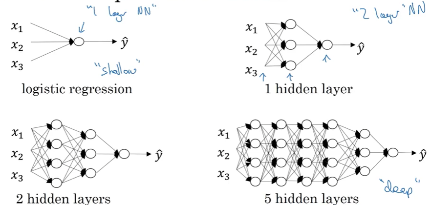
Defining Depth

A neural network’s depth refers to the number of layers:

Architecture	Layers	Classification
Logistic Regression	$L = 1$	Very shallow (no hidden layers)
1 Hidden Layer	$L = 2$	Shallow neural network
2 Hidden Layers	$L = 3$	Deep neural network
5 Hidden Layers	$L = 6$	Deep neural network
100+ Hidden Layers	$L \geq 100$	Very deep (ResNet, Transformers)

Shallow vs Deep

Shallow models (Week 1-3):

Input → Hidden Layer → Output

Deep models (Week 4):

Input → Hidden 1 → Hidden 2 → Hidden 3 → ... → Output

Why Deep Networks Are Powerful

Over the past several years, the AI and machine learning community has discovered that very deep neural networks can learn functions that shallower models cannot.

Key insights:

Deep networks learn hierarchical representations
Each layer builds on features from previous layers
More layers = more complex patterns can be learned

However, for any given problem, it’s hard to predict in advance exactly how deep your network should be.

Depth as a Hyperparameter

The number of hidden layers is a hyperparameter you should experiment with:

Recommended approach:

Try logistic regression ($L = 1$)
Try 1 hidden layer ($L = 2$)
Try 2 hidden layers ($L = 3$)
Evaluate performance on validation/dev set
Choose the architecture that performs best

Note: We’ll discuss validation sets and hyperparameter tuning in detail later in the course.

Notation for Deep Networks

Example: 4-Layer Network

Consider this network architecture:

Architecture details:

Layer 0 (input): 3 features
Layer 1 (hidden): 5 units
Layer 2 (hidden): 5 units
Layer 3 (hidden): 3 units
Layer 4 (output): 1 unit

Core Notation

We use the following symbols to describe deep networks:

Symbol	Meaning	Example for Our Network
$L$	Total number of layers	$L = 4$
$n^{[l]}$	Number of units in layer $l$	$n^{[1]} = 5$, $n^{[2]} = 5$, $n^{[3]} = 3$
$a^{[l]}$	Activations in layer $l$	$a^{[1]}$ has 5 values
$W^{[l]}$	Weights for layer $l$	$W^{[1]}$ connects layer 0 to layer 1
$b^{[l]}$	Biases for layer $l$	$b^{[2]}$ has 5 values
$Z^{[l]}$	Linear output of layer $l$	$Z^{[l]} = W^{[l]} a^{[l-1]} + b^{[l]}$

Layer Indexing Convention

Important: We index the input layer as layer 0, but don’t count it when describing network depth.

For our 4-layer network:

Layer 0: Input ($n^{[0]} = 3$)
Layer 1: First hidden layer ($n^{[1]} = 5$)
Layer 2: Second hidden layer ($n^{[2]} = 5$)
Layer 3: Third hidden layer ($n^{[3]} = 3$)
Layer 4: Output layer ($n^{[4]} = 1$)

We say this is a “4-layer network” because $L = 4$ (not counting the input).

Detailed Example: Unit Counts

Let’s walk through each layer:

Input layer (layer 0):

\[n^{[0]} = n_x = 3\]

(3 input features)

First hidden layer (layer 1):

\[n^{[1]} = 5\]

(5 hidden units in layer 1)

Second hidden layer (layer 2):

\[n^{[2]} = 5\]

(5 hidden units in layer 2)

Third hidden layer (layer 3):

\[n^{[3]} = 3\]

(3 hidden units in layer 3)

Output layer (layer 4):

\[n^{[4]} = n^{[L]} = 1\]

(1 output unit, since $L = 4$)

Activation Notation

Activations for Each Layer

For each layer $l$, we compute activations $a^{[l]}$:

\[a^{[l]} = g^{[l]}(Z^{[l]})\]

where $g^{[l]}$ is the activation function for layer $l$.

During forward propagation:

Compute linear combination: $Z^{[l]} = W^{[l]} a^{[l-1]} + b^{[l]}$
Apply activation function: $a^{[l]} = g^{[l]}(Z^{[l]})$

Special Cases

Input layer (layer 0):

\[a^{[0]} = X\]

The input features $X$ are the “activations” of layer 0.

Output layer (layer $L$):

\[a^{[L]} = \hat{y}\]

The activations of the final layer are the network’s predictions.

Summary of Activation Notation

\[\boxed{\begin{align} a^{[0]} &= X \quad \text{(input features)} \\ a^{[1]}, a^{[2]}, \ldots, a^{[L-1]} &= \text{hidden layer activations} \\ a^{[L]} &= \hat{y} \quad \text{(predictions)} \end{align}}\]

Parameter Notation

Weights and Biases

For each layer $l$, we have two sets of parameters:

Weight matrix $W^{[l]}$:

Connects layer $l-1$ to layer $l$
Shape: $(n^{[l]}, n^{[l-1]})$

Bias vector $b^{[l]}$:

One bias per unit in layer $l$
Shape: $(n^{[l]}, 1)$

Computing Linear Outputs

For layer $l$:

\[Z^{[l]} = W^{[l]} a^{[l-1]} + b^{[l]}\]

Where:

$W^{[l]}$ are the weights for layer $l$
$a^{[l-1]}$ are activations from the previous layer
$b^{[l]}$ are the biases for layer $l$

Complete Forward Propagation

Putting it all together:

\[\boxed{\begin{align} Z^{[l]} &= W^{[l]} a^{[l-1]} + b^{[l]} \\ a^{[l]} &= g^{[l]}(Z^{[l]}) \end{align}}\]

Repeat for $l = 1, 2, \ldots, L$.

Notation Reference Table

Here’s a complete summary of the notation we use for deep networks:

Symbol	Meaning	Type	Example Value
$L$	Number of layers	Scalar	$L = 4$
$n^{[l]}$	Units in layer $l$	Scalar	$n^{[2]} = 5$
$n^{[0]}$	Input features	Scalar	$n^{[0]} = 3$
$n^{[L]}$	Output units	Scalar	$n^{[L]} = 1$
$a^{[l]}$	Activations of layer $l$	Vector/Matrix	Shape $(n^{[l]}, m)$
$a^{[0]}$	Input features	Matrix	$a^{[0]} = X$
$a^{[L]}$	Predictions	Vector/Matrix	$a^{[L]} = \hat{y}$
$W^{[l]}$	Weights for layer $l$	Matrix	Shape $(n^{[l]}, n^{[l-1]})$
$b^{[l]}$	Biases for layer $l$	Vector	Shape $(n^{[l]}, 1)$
$Z^{[l]}$	Linear output of layer $l$	Vector/Matrix	Shape $(n^{[l]}, m)$
$g^{[l]}$	Activation function for layer $l$	Function	ReLU, sigmoid, tanh

Tip: If you forget what a symbol means, refer back to this table or the course notation guide!

Example: Computing Dimensions

For our 4-layer network with $m = 100$ training examples:

Layer Dimensions

Layer	$n^{[l]}$	$W^{[l]}$ shape	$b^{[l]}$ shape	$a^{[l]}$ shape	$Z^{[l]}$ shape
0 (input)	3	-	-	$(3, 100)$	-
1 (hidden)	5	$(5, 3)$	$(5, 1)$	$(5, 100)$	$(5, 100)$
2 (hidden)	5	$(5, 5)$	$(5, 1)$	$(5, 100)$	$(5, 100)$
3 (hidden)	3	$(3, 5)$	$(3, 1)$	$(3, 100)$	$(3, 100)$
4 (output)	1	$(1, 3)$	$(1, 1)$	$(1, 100)$	$(1, 100)$

Parameter Count

Total parameters in this network:

\[\begin{align} W^{[1]}: &\quad 5 \times 3 = 15 \\ b^{[1]}: &\quad 5 \\ W^{[2]}: &\quad 5 \times 5 = 25 \\ b^{[2]}: &\quad 5 \\ W^{[3]}: &\quad 3 \times 5 = 15 \\ b^{[3]}: &\quad 3 \\ W^{[4]}: &\quad 1 \times 3 = 3 \\ b^{[4]}: &\quad 1 \\ \hline \text{Total}: &\quad \boxed{72 \text{ parameters}} \end{align}\]

Visual Architecture Diagram

Forward propagation flow:

$a^{[0]} = X$ (input)
$Z^{[1]} = W^{[1]} a^{[0]} + b^{[1]}$, then $a^{[1]} = g^{[1]}(Z^{[1]})$
$Z^{[2]} = W^{[2]} a^{[1]} + b^{[2]}$, then $a^{[2]} = g^{[2]}(Z^{[2]})$
$Z^{[3]} = W^{[3]} a^{[2]} + b^{[3]}$, then $a^{[3]} = g^{[3]}(Z^{[3]})$
$Z^{[4]} = W^{[4]} a^{[3]} + b^{[4]}$, then $a^{[4]} = g^{[4]}(Z^{[4]}) = \hat{y}$

Key Takeaways

Deep networks have multiple hidden layers ($L \geq 2$)
$L$ denotes total number of layers (not counting input)
$n^{[l]}$ is the number of units in layer $l$
Layer indexing: Input is layer 0, layers 1 through $L$ are counted
$a^{[l]}$ represents activations of layer $l$
$W^{[l]}$ and $b^{[l]}$ are parameters for layer $l$
$a^{[0]} = X$ (input features)
$a^{[L]} = \hat{y}$ (predictions)
Superscript $[l]$ always denotes layer number
Forward propagation: $Z^{[l]} = W^{[l]} a^{[l-1]} + b^{[l]}$, then $a^{[l]} = g^{[l]}(Z^{[l]})$
Depth is a hyperparameter - experiment to find optimal value
Deep networks are more powerful than shallow ones for many tasks
Notation guide available - refer to it whenever needed
Matrix dimensions: $W^{[l]}$ is $(n^{[l]}, n^{[l-1]})$, $b^{[l]}$ is $(n^{[l]}, 1)$
Each layer builds on previous - hierarchical feature learning

Deep L-layer Neural Network

Table of contents