Last modified: Jan 31 2026 at 10:09 PM • 5 mins read
Vectorizing Across Multiple Examples
Table of contents
- Introduction
- Review: Single Example Forward Propagation
- The Problem: Multiple Examples
- Non-Vectorized Implementation (Slow)
- Vectorized Implementation (Fast)
- Implementation
- Understanding Matrix Dimensions
- How to Think About Matrix Layout
- Comparison: For-Loop vs Vectorized
- Why This Works
- Key Takeaways
Introduction
In the previous lesson, we learned how to compute predictions for a single training example. Now we’ll vectorize across multiple training examples to process the entire dataset simultaneously - similar to what we did for logistic regression.
By stacking training examples as columns in a matrix, we can transform our 4 equations with minimal changes to compute outputs for all examples at once.
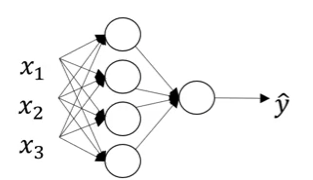
Review: Single Example Forward Propagation
For a single training example $x$, we computed:
\[z^{[1]} = W^{[1]} x + b^{[1]}\] \[a^{[1]} = \sigma(z^{[1]})\] \[z^{[2]} = W^{[2]} a^{[1]} + b^{[2]}\] \[a^{[2]} = \sigma(z^{[2]}) = \hat{y}\]The Problem: Multiple Examples
With $m$ training examples, we need predictions for each:
\[x^{(1)} \rightarrow \hat{y}^{(1)} = a^{[2](1)}\] \[x^{(2)} \rightarrow \hat{y}^{(2)} = a^{[2](2)}\] \[\vdots\] \[x^{(m)} \rightarrow \hat{y}^{(m)} = a^{[2](m)}\]Notation Clarification
\[a^{[l](i)}\]- Square brackets $[l]$: layer number
- Round brackets $(i)$: training example number
So $a^{2}$ means “activation from layer 2 for training example 3”.
Non-Vectorized Implementation (Slow)
The naive approach uses a for-loop:
for i in range(m):
    # Hidden layer
    z[1](i) = W[1] @ x(i) + b[1]
    a[1](i) = sigmoid(z[1](i))

    # Output layer
    z[2](i) = W[2] @ a[1](i) + b[2]
    a[2](i) = sigmoid(z[2](i))
Problem: Processing one example at a time is inefficient. Let’s vectorize!
Vectorized Implementation (Fast)
Step 1: Stack Training Examples as Columns
Create the input matrix $X$ by stacking examples horizontally:
\[X = \begin{bmatrix} | & | & & | \\ x^{(1)} & x^{(2)} & \cdots & x^{(m)} \\ | & | & & | \end{bmatrix}\]Shape: $(n_x, m)$ where $n_x$ = number of features, $m$ = number of examples
Step 2: Use Capital Letter Matrices
Replace lowercase vectors with uppercase matrices:
Single example notation:
\[x, \quad z^{[1]}, \quad a^{[1]}, \quad z^{[2]}, \quad a^{[2]}\]Multiple examples notation (stacked as columns):
\[X = [x^{(1)} \ x^{(2)} \ \cdots \ x^{(m)}], \quad \text{shape: } (n_x, m)\] \[Z^{[1]} = [z^{[1](1)} \ z^{[1](2)} \ \cdots \ z^{[1](m)}], \quad \text{shape: } (n^{[1]}, m)\] \[A^{[1]} = [a^{[1](1)} \ a^{[1](2)} \ \cdots \ a^{[1](m)}], \quad \text{shape: } (n^{[1]}, m)\] \[Z^{[2]} = [z^{[2](1)} \ z^{[2](2)} \ \cdots \ z^{[2](m)}], \quad \text{shape: } (n^{[2]}, m)\] \[A^{[2]} = [a^{[2](1)} \ a^{[2](2)} \ \cdots \ a^{[2](m)}], \quad \text{shape: } (n^{[2]}, m)\]Step 3: Vectorized Forward Propagation
Simply replace lowercase with uppercase:
\[Z^{[1]} = W^{[1]} X + b^{[1]}\] \[A^{[1]} = \sigma(Z^{[1]})\] \[Z^{[2]} = W^{[2]} A^{[1]} + b^{[2]}\] \[A^{[2]} = \sigma(Z^{[2]})\]That’s it! The same 4 equations, just with capital letters.
Implementation
# Vectorized forward propagation for m examples
# Hidden layer
Z1 = np.dot(W1, X) + b1      # Shape: (4, m)
A1 = sigmoid(Z1)              # Shape: (4, m)

# Output layer
Z2 = np.dot(W2, A1) + b2     # Shape: (1, m)
A2 = sigmoid(Z2)              # Shape: (1, m)

# A2 contains predictions for all m examples
y_hat = A2
Understanding Matrix Dimensions
Let’s verify with $n_x = 3$ features, $n^{[1]} = 4$ hidden units, and $m = 100$ examples:
| Computation | Dimensions | Result |
|---|---|---|
| $W^{[1]} X$ | $(4 \times 3) \cdot (3 \times 100)$ | $(4 \times 100)$ |
| $Z^{[1]} = W^{[1]} X + b^{[1]}$ | $(4 \times 100) + (4 \times 1)$ | $(4 \times 100)$ |
| $A^{[1]} = \sigma(Z^{[1]})$ | $\sigma((4 \times 100))$ | $(4 \times 100)$ |
| $W^{[2]} A^{[1]}$ | $(1 \times 4) \cdot (4 \times 100)$ | $(1 \times 100)$ |
| $Z^{[2]} = W^{[2]} A^{[1]} + b^{[2]}$ | $(1 \times 100) + (1 \times 1)$ | $(1 \times 100)$ |
| $A^{[2]} = \sigma(Z^{[2]})$ | $\sigma((1 \times 100))$ | $(1 \times 100)$ |
Note: Broadcasting automatically handles adding $b^{[1]}$ (shape $(4,1)$) to each column of the $(4, 100)$ matrix.
How to Think About Matrix Layout
Horizontal Axis: Training Examples
Moving left to right across columns = scanning through training examples.
Vertical Axis: Nodes/Features
Moving top to bottom down rows = scanning through nodes (or features).
Example: Matrix $A^{[1]}$ with 4 Hidden Units and 5 Examples
\[A^{[1]} = \begin{bmatrix} a^{[1](1)}_1 & a^{[1](2)}_1 & a^{[1](3)}_1 & a^{[1](4)}_1 & a^{[1](5)}_1 \\ a^{[1](1)}_2 & a^{[1](2)}_2 & a^{[1](3)}_2 & a^{[1](4)}_2 & a^{[1](5)}_2 \\ a^{[1](1)}_3 & a^{[1](2)}_3 & a^{[1](3)}_3 & a^{[1](4)}_3 & a^{[1](5)}_3 \\ a^{[1](1)}_4 & a^{[1](2)}_4 & a^{[1](3)}_4 & a^{[1](4)}_4 & a^{[1](5)}_4 \end{bmatrix}\]Interpretation:
- Top-left $a^{1}_1$: Activation of hidden unit 1 on example 1
- Moving down: Hidden unit 2, 3, 4 on example 1
- Moving right: Hidden unit 1 on examples 2, 3, 4, 5
- Bottom-right $a^{1}_4$: Activation of hidden unit 4 on example 5
Same Pattern for All Matrices
| Matrix | Rows (vertical) | Columns (horizontal) |
|---|---|---|
| $X$ | Input features ($x_1, x_2, \ldots, x_{n_x}$) | Training examples |
| $Z^{[1]}, A^{[1]}$ | Hidden units (nodes 1, 2, 3, 4) | Training examples |
| $Z^{[2]}, A^{[2]}$ | Output units | Training examples |
Comparison: For-Loop vs Vectorized
Non-Vectorized (Slow)
# Process one example at a time
for i in range(m):
    z1_i = np.dot(W1, x_i) + b1
    a1_i = sigmoid(z1_i)
    z2_i = np.dot(W2, a1_i) + b2
    a2_i = sigmoid(z2_i)
Time: $O(m)$ iterations
Vectorized (Fast)
# Process all examples simultaneously
Z1 = np.dot(W1, X) + b1
A1 = sigmoid(Z1)
Z2 = np.dot(W2, A1) + b2
A2 = sigmoid(Z2)
Time: $O(1)$ operation (parallelized)
Why This Works
The vectorization works because matrix multiplication naturally implements the “loop” over training examples:
\[W^{[1]} X = W^{[1]} \begin{bmatrix} x^{(1)} & x^{(2)} & \cdots & x^{(m)} \end{bmatrix} = \begin{bmatrix} W^{[1]} x^{(1)} & W^{[1]} x^{(2)} & \cdots & W^{[1]} x^{(m)} \end{bmatrix}\]Each column of the result corresponds to processing one training example - exactly what the for-loop did, but computed in parallel!
Key Takeaways
- Stack training examples as columns to create matrices $X$, $Z^{[l]}$, $A^{[l]}$
- Replace lowercase with uppercase: $x \rightarrow X$, $z^{[l]} \rightarrow Z^{[l]}$, $a^{[l]} \rightarrow A^{[l]}$
- Same 4 equations work for both single and multiple examples (just change case)
- Matrix dimensions: $(n^{[l]}, m)$ where $n^{[l]}$ = units in layer $l$, $m$ = examples
- Horizontal (columns): Different training examples
- Vertical (rows): Different nodes/features in the layer
- Broadcasting handles adding bias vectors to matrices automatically
- Vectorization eliminates for-loops and leverages parallel computation