Last modified: Jan 31 2026 at 10:09 PM • 5 mins read
Explanation for Vectorized Implementation
Table of contents
- Introduction
- The Core Question
- Step-by-Step Derivation
- Matrix Form: Stacking Examples
- Adding Back the Bias
- Generalizing to All Layers
- Complete Recap
- Symmetry in Neural Network Layers
- Key Takeaways
Introduction
In the previous lesson, we saw how to vectorize forward propagation by stacking training examples as columns in matrix $X$. Now let’s provide a mathematical justification for why this vectorization is correct.
The Core Question
Why does this equation work for multiple examples?
\[Z^{[1]} = W^{[1]} X + b^{[1]}\]Let’s prove it step by step.
Step-by-Step Derivation
Individual Example Computations
For individual training examples, we compute:
Example 1:
\[z^{[1](1)} = W^{[1]} x^{(1)} + b^{[1]}\]Example 2:
\[z^{[1](2)} = W^{[1]} x^{(2)} + b^{[1]}\]Example 3:
\[z^{[1](3)} = W^{[1]} x^{(3)} + b^{[1]}\]Simplification: Ignoring Bias (Temporarily)
To make the explanation clearer, let’s temporarily assume $b^{[1]} = 0$. We’ll add it back later:
\[z^{[1](1)} = W^{[1]} x^{(1)}\] \[z^{[1](2)} = W^{[1]} x^{(2)}\] \[z^{[1](3)} = W^{[1]} x^{(3)}\]Understanding the Matrix Multiplication
Each computation produces a column vector:
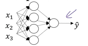
\[W^{[1]} x^{(1)} = \text{column vector}\] \[W^{[1]} x^{(2)} = \text{column vector}\] \[W^{[1]} x^{(3)} = \text{column vector}\]For example, if $W^{[1]}$ has shape $(4, 3)$ and $x^{(i)}$ has shape $(3, 1)$, then each result is a $(4, 1)$ column vector.
Matrix Form: Stacking Examples
Building Matrix $X$
Now, create matrix $X$ by stacking examples as columns:
\[X = \begin{bmatrix} | & | & | \\ x^{(1)} & x^{(2)} & x^{(3)} \\ | & | & | \end{bmatrix}\]Shape: $(n_x, 3)$ for 3 examples with $n_x$ features.
Computing $W^{[1]} X$
When we multiply $W^{[1]} X$, matrix multiplication produces:
\[W^{[1]} X = W^{[1]} \begin{bmatrix} | & | & | \\ x^{(1)} & x^{(2)} & x^{(3)} \\ | & | & | \end{bmatrix} = \begin{bmatrix} | & | & | \\ W^{[1]} x^{(1)} & W^{[1]} x^{(2)} & W^{[1]} x^{(3)} \\ | & | & | \end{bmatrix}\]Key insight: Matrix multiplication applies $W^{[1]}$ to each column of $X$ independently!
Result is $Z^{[1]}$
The result is exactly the matrix $Z^{[1]}$:
\[Z^{[1]} = \begin{bmatrix} | & | & | \\ z^{[1](1)} & z^{[1](2)} & z^{[1](3)} \\ | & | & | \end{bmatrix}\]where each column is the result for one training example.
Adding Back the Bias
Python Broadcasting
When we add $b^{[1]}$ back:
\[Z^{[1]} = W^{[1]} X + b^{[1]}\]Python’s broadcasting automatically adds $b^{[1]}$ to each column of $W^{[1]} X$.
How Broadcasting Works
If $b^{[1]}$ has shape $(4, 1)$ and $W^{[1]} X$ has shape $(4, 3)$:
\[\begin{bmatrix} w_{11}x^{(1)}_1 + \cdots & w_{11}x^{(2)}_1 + \cdots & w_{11}x^{(3)}_1 + \cdots \\ w_{21}x^{(1)}_1 + \cdots & w_{21}x^{(2)}_1 + \cdots & w_{21}x^{(3)}_1 + \cdots \\ w_{31}x^{(1)}_1 + \cdots & w_{31}x^{(2)}_1 + \cdots & w_{31}x^{(3)}_1 + \cdots \\ w_{41}x^{(1)}_1 + \cdots & w_{41}x^{(2)}_1 + \cdots & w_{41}x^{(3)}_1 + \cdots \end{bmatrix} + \begin{bmatrix} b_1 \\ b_2 \\ b_3 \\ b_4 \end{bmatrix}\]becomes:
\[\begin{bmatrix} (\cdots) + b_1 & (\cdots) + b_1 & (\cdots) + b_1 \\ (\cdots) + b_2 & (\cdots) + b_2 & (\cdots) + b_2 \\ (\cdots) + b_3 & (\cdots) + b_3 & (\cdots) + b_3 \\ (\cdots) + b_4 & (\cdots) + b_4 & (\cdots) + b_4 \end{bmatrix}\]Broadcasting adds $b^{[1]}$ to every column automatically!
Generalizing to All Layers
The same logic applies to all four equations:
For-Loop Version (Non-Vectorized)
for i in range(m):
    z[1](i) = W[1] @ x(i) + b[1]
    a[1](i) = sigmoid(z[1](i))
    z[2](i) = W[2] @ a[1](i) + b[2]
    a[2](i) = sigmoid(z[2](i))
Vectorized Version
Z1 = np.dot(W1, X) + b1
A1 = sigmoid(Z1)
Z2 = np.dot(W2, A1) + b2
A2 = sigmoid(Z2)
Each equation works by the same principle:
- Stack inputs as columns in a matrix
- Matrix multiplication processes all columns simultaneously
- Broadcasting adds bias to all columns
- Element-wise operations (like sigmoid) apply to each element
Complete Recap

Non-Vectorized (One Example at a Time)
\[\text{for } i = 1 \text{ to } m:\] \[z^{[1](i)} = W^{[1]} x^{(i)} + b^{[1]}\] \[a^{[1](i)} = \sigma(z^{[1](i)})\] \[z^{[2](i)} = W^{[2]} a^{[1](i)} + b^{[2]}\] \[a^{[2](i)} = \sigma(z^{[2](i)})\]Vectorized (All Examples Simultaneously)
Stack examples as columns:
\[X = [x^{(1)} \ x^{(2)} \ \cdots \ x^{(m)}]\] \[Z^{[1]} = [z^{[1](1)} \ z^{[1](2)} \ \cdots \ z^{[1](m)}]\] \[A^{[1]} = [a^{[1](1)} \ a^{[1](2)} \ \cdots \ a^{[1](m)}]\] \[Z^{[2]} = [z^{[2](1)} \ z^{[2](2)} \ \cdots \ z^{[2](m)}]\] \[A^{[2]} = [a^{[2](1)} \ a^{[2](2)} \ \cdots \ a^{[2](m)}]\]Then compute:
\[Z^{[1]} = W^{[1]} X + b^{[1]}\] \[A^{[1]} = \sigma(Z^{[1]})\] \[Z^{[2]} = W^{[2]} A^{[1]} + b^{[2]}\] \[A^{[2]} = \sigma(Z^{[2]})\]Symmetry in Neural Network Layers
Notation: $X = A^{[0]}$
Recall that the input features can be written as:
\[X = A^{[0]}\]This means $x^{(i)} = a^{0}$ for each training example.
Layer 1 Equations
\[Z^{[1]} = W^{[1]} A^{[0]} + b^{[1]}\] \[A^{[1]} = \sigma(Z^{[1]})\]Layer 2 Equations
\[Z^{[2]} = W^{[2]} A^{[1]} + b^{[2]}\] \[A^{[2]} = \sigma(Z^{[2]})\]Pattern Recognition
Notice the repeating pattern:
\[Z^{[l]} = W^{[l]} A^{[l-1]} + b^{[l]}\] \[A^{[l]} = \sigma(Z^{[l]})\]Each layer performs the same computation:
- Linear transformation: $Z^{[l]} = W^{[l]} A^{[l-1]} + b^{[l]}$
- Non-linear activation: $A^{[l]} = \sigma(Z^{[l]})$
This pattern extends to deep neural networks with many layers - each layer just repeats these two steps!
Key Takeaways
- Matrix multiplication naturally implements the “loop” over training examples
- Broadcasting adds bias vectors to all columns automatically
- Stacking as columns: $X = [x^{(1)} \ x^{(2)} \ \cdots \ x^{(m)}]$ enables vectorization
- All four equations vectorize the same way - stack inputs, apply operations
- Neural network layers follow a repeating pattern: $Z^{[l]} = W^{[l]} A^{[l-1]} + b^{[l]}$, then $A^{[l]} = \sigma(Z^{[l]})$
- Deep networks just repeat this pattern more times
- Vectorization is mathematically equivalent to for-loops but much faster