Last modified: Jan 31 2026 at 10:09 PM • 8 mins read

Derivatives of Activation Functions

Table of contents

1. Introduction
2. Notation
3. 1. Sigmoid Function Derivative
4. 2. Tanh Function Derivative
5. 3. ReLU Function Derivative
6. 4. Leaky ReLU Function Derivative
7. Summary Table
8. Comparison of Gradient Properties
9. Complete Implementation Example
10. Why We Need These Derivatives
11. Key Takeaways

---

Introduction

To implement backpropagation for training neural networks, we need to compute the derivatives (slopes) of activation functions. This lesson covers how to calculate derivatives for the most common activation functions used in neural networks.

Notation

Derivative Notation

For an activation function $g(z)$, we use multiple equivalent notations for its derivative:

\[\frac{d}{dz} g(z) = g'(z) = \frac{dg}{dz}\]

where:

• $g’(z)$ is called “g prime of z” (common shorthand)
• Represents the slope of $g(z)$ at point $z$

In Terms of Activations

If $a = g(z)$, we can often express $g’(z)$ in terms of $a$:

\[g'(z) = f(a)\]

This is computationally efficient because we’ve already computed $a$ during forward propagation!

1. Sigmoid Function Derivative

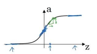
Function

\[g(z) = \sigma(z) = \frac{1}{1 + e^{-z}}\]

Derivative Formula

\[g'(z) = \frac{d}{dz} \sigma(z) = g(z) \cdot (1 - g(z))\]

Or equivalently, since $a = g(z)$:

\[g'(z) = a \cdot (1 - a)\]

Verification at Key Points

Let’s verify this formula makes sense:

Case 1: $z = 10$ (very large)

\[g(10) \approx 1\] \[g'(10) = 1 \cdot (1 - 1) = 0 \quad \checkmark\]

✅ Correct! The sigmoid function is flat (slope ≈ 0) for large positive $z$.

Case 2: $z = -10$ (very small)

\[g(-10) \approx 0\] \[g'(-10) = 0 \cdot (1 - 0) = 0 \quad \checkmark\]

✅ Correct! The sigmoid function is also flat for large negative $z$.

Case 3: $z = 0$ (middle)

\[g(0) = 0.5\] \[g'(0) = 0.5 \cdot (1 - 0.5) = 0.25 \quad \checkmark\]

✅ Correct! Maximum slope occurs at $z = 0$.

Implementation

def sigmoid(z):
    """Sigmoid activation function"""
    return 1 / (1 + np.exp(-z))

def sigmoid_derivative(z):
    """Derivative of sigmoid function"""
    a = sigmoid(z)
    return a * (1 - a)

# Alternative: if you already have 'a' computed
def sigmoid_derivative_from_a(a):
    """Derivative using already-computed activation"""
    return a * (1 - a)

Gradient Flow Characteristics

Problem: Sigmoid has vanishing gradient issue

• When $|z|$ is large, $g’(z) \approx 0$
• Gradient becomes very small, slowing learning
• Maximum derivative is only $0.25$ at $z = 0$

2. Tanh Function Derivative

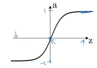
Function

\[g(z) = \tanh(z) = \frac{e^z - e^{-z}}{e^z + e^{-z}}\]

Range: $(-1, 1)$

Derivative Formula

\[g'(z) = \frac{d}{dz} \tanh(z) = 1 - (g(z))^2\]

Or equivalently, since $a = g(z)$:

\[g'(z) = 1 - a^2\]

Verification at Key Points

Case 1: $z = 10$ (very large)

\[\tanh(10) \approx 1\] \[g'(10) = 1 - 1^2 = 0 \quad \checkmark\]

✅ Function is flat for large positive $z$.

Case 2: $z = -10$ (very small)

\[\tanh(-10) \approx -1\] \[g'(-10) = 1 - (-1)^2 = 1 - 1 = 0 \quad \checkmark\]

✅ Function is flat for large negative $z$.

Case 3: $z = 0$ (middle)

\[\tanh(0) = 0\] \[g'(0) = 1 - 0^2 = 1 \quad \checkmark\]

✅ Maximum slope occurs at $z = 0$.

Implementation

def tanh(z):
    """Hyperbolic tangent activation function"""
    return np.tanh(z)

def tanh_derivative(z):
    """Derivative of tanh function"""
    a = np.tanh(z)
    return 1 - a**2

# Alternative: if you already have 'a' computed
def tanh_derivative_from_a(a):
    """Derivative using already-computed activation"""
    return 1 - a**2

Gradient Flow Characteristics

Better than sigmoid but still has issues:

• Maximum derivative is $1$ at $z = 0$ (better than sigmoid’s $0.25$)

• Still suffers from vanishing gradient for $

  z

  $ large

• Zero-centered outputs help with gradient flow

3. ReLU Function Derivative

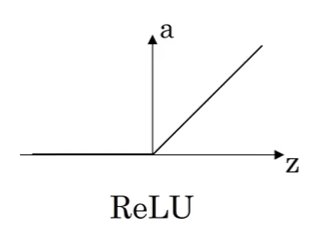
Function

\[g(z) = \text{ReLU}(z) = \max(0, z) = \begin{cases} z & \text{if } z > 0 \\ 0 & \text{if } z \leq 0 \end{cases}\]

Derivative Formula

\[g'(z) = \begin{cases} 1 & \text{if } z > 0 \\ 0 & \text{if } z < 0 \\ \text{undefined} & \text{if } z = 0 \end{cases}\]

Handling the Discontinuity at $z = 0$

Mathematical Issue: Derivative is technically undefined at $z = 0$.

Practical Solution: In implementation, set $g’(0)$ to either $0$ or $1$ - it doesn’t matter!

Why it doesn’t matter:

1. The probability of $z$ being exactly $0.000000…$ is infinitesimally small
2. For optimization experts: $g’$ becomes a sub-gradient, and gradient descent still works
3. In practice, this choice has negligible impact on training

Common convention: Set $g’(0) = 1$

Implementation

def relu(z):
    """ReLU activation function"""
    return np.maximum(0, z)

def relu_derivative(z):
    """Derivative of ReLU function"""
    return (z > 0).astype(float)
    # Returns 1 where z > 0, and 0 where z <= 0

# Alternative explicit form
def relu_derivative_explicit(z):
    """Derivative of ReLU - explicit conditionals"""
    dz = np.zeros_like(z)
    dz[z > 0] = 1
    return dz

Gradient Flow Characteristics

Advantages:

• ✅ No vanishing gradient for $z > 0$ (gradient = 1)
• ✅ Computationally efficient
• ✅ Sparse activation (many neurons output 0)

Disadvantages:

• ❌ “Dying ReLU” problem: neurons with $z < 0$ have zero gradient
• ❌ Not differentiable at $z = 0$

4. Leaky ReLU Function Derivative

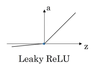
Function

\[g(z) = \text{Leaky ReLU}(z) = \max(\alpha z, z) = \begin{cases} z & \text{if } z > 0 \\ \alpha z & \text{if } z \leq 0 \end{cases}\]

where $\alpha$ is a small constant (typically $\alpha = 0.01$)

Derivative Formula

\[g'(z) = \begin{cases} 1 & \text{if } z > 0 \\ \alpha & \text{if } z < 0 \\ \text{undefined} & \text{if } z = 0 \end{cases}\]

Handling the Discontinuity

Same as ReLU: set $g’(0)$ to either $\alpha$ or $1$ - it doesn’t matter in practice.

Common convention: Set $g’(0) = 1$

Implementation

def leaky_relu(z, alpha=0.01):
    """Leaky ReLU activation function"""
    return np.maximum(alpha * z, z)

def leaky_relu_derivative(z, alpha=0.01):
    """Derivative of Leaky ReLU function"""
    dz = np.ones_like(z)
    dz[z < 0] = alpha
    return dz

# Alternative vectorized form
def leaky_relu_derivative_vectorized(z, alpha=0.01):
    """Derivative - vectorized version"""
    return np.where(z > 0, 1, alpha)

Gradient Flow Characteristics

Advantages over ReLU:

• ✅ No “dying ReLU” problem - gradient is $\alpha$ (not 0) for $z < 0$
• ✅ Allows negative values to have small gradient
• ✅ All benefits of ReLU plus gradient flow for negative values

Summary Table

Activation	Function	Derivative $g’(z)$	Derivative in terms of $a$	At $z=0$
Sigmoid	$\frac{1}{1+e^{-z}}$	$g(z)(1-g(z))$	$a(1-a)$	$0.25$
Tanh	$\frac{e^z-e^{-z}}{e^z+e^{-z}}$	$1-(g(z))^2$	$1-a^2$	$1$
ReLU	$\max(0,z)$	$\begin{cases} 1 & z>0 \ 0 & z\leq0 \end{cases}$	N/A	$0$ or $1$
Leaky ReLU	$\max(\alpha z,z)$	$\begin{cases} 1 & z>0 \ \alpha & z\leq0 \end{cases}$	N/A	$\alpha$ or $1$

Comparison of Gradient Properties

Maximum Gradient Values

\[\max g'(z) = \begin{cases} 0.25 & \text{Sigmoid} \\ 1 & \text{Tanh} \\ 1 & \text{ReLU} \\ 1 & \text{Leaky ReLU} \end{cases}\]

Implication: Sigmoid’s small maximum gradient makes it slowest to train.

Vanishing Gradient Problem

Affected: Sigmoid, Tanh

• Gradients approach 0 for $

  z

  $ large

• Slows learning significantly

Not affected: ReLU, Leaky ReLU

• Constant gradient for positive values
• Faster training in practice

Complete Implementation Example

import numpy as np

class ActivationFunctions:
    """Collection of activation functions and their derivatives"""

    @staticmethod
    def sigmoid(z):
        return 1 / (1 + np.exp(-z))

    @staticmethod
    def sigmoid_derivative(a):
        """Derivative using already-computed activation"""
        return a * (1 - a)

    @staticmethod
    def tanh(z):
        return np.tanh(z)

    @staticmethod
    def tanh_derivative(a):
        """Derivative using already-computed activation"""
        return 1 - a**2

    @staticmethod
    def relu(z):
        return np.maximum(0, z)

    @staticmethod
    def relu_derivative(z):
        return (z > 0).astype(float)

    @staticmethod
    def leaky_relu(z, alpha=0.01):
        return np.maximum(alpha * z, z)

    @staticmethod
    def leaky_relu_derivative(z, alpha=0.01):
        dz = np.ones_like(z)
        dz[z < 0] = alpha
        return dz

# Example usage
z = np.array([-2, -1, 0, 1, 2])
act = ActivationFunctions()

print("Sigmoid:")
print("  Values:", act.sigmoid(z))
print("  Derivatives:", act.sigmoid_derivative(act.sigmoid(z)))

print("\nTanh:")
print("  Values:", act.tanh(z))
print("  Derivatives:", act.tanh_derivative(act.tanh(z)))

print("\nReLU:")
print("  Values:", act.relu(z))
print("  Derivatives:", act.relu_derivative(z))

print("\nLeaky ReLU:")
print("  Values:", act.leaky_relu(z))
print("  Derivatives:", act.leaky_relu_derivative(z))

Why We Need These Derivatives

During backpropagation, we compute gradients by applying the chain rule:

\[\frac{\partial \mathcal{L}}{\partial z^{[l]}} = \frac{\partial \mathcal{L}}{\partial a^{[l]}} \cdot \frac{\partial a^{[l]}}{\partial z^{[l]}}\]

where $\frac{\partial a^{[l]}}{\partial z^{[l]}} = g’(z^{[l]})$ is the activation function derivative!

These derivatives are essential for:

1. Computing gradients in backpropagation
2. Updating weights and biases
3. Training the neural network

Key Takeaways

1. Derivative notation: $g’(z) = \frac{d}{dz} g(z)$ represents the slope of activation function
2. Sigmoid derivative: $g’(z) = a(1-a)$ - convenient to compute from activation
3. Tanh derivative: $g’(z) = 1 - a^2$ - also convenient to compute from activation
4. ReLU derivative: $g’(z) = 1$ if $z > 0$, else $0$ - simple to compute
5. Leaky ReLU derivative: $g’(z) = 1$ if $z > 0$, else $\alpha$ - fixes dying ReLU
6. Discontinuity at zero: For ReLU variants, set $g’(0)$ to any value (doesn’t matter)
7. Vanishing gradient: Sigmoid and tanh suffer from this; ReLU variants don’t
8. Computational efficiency: Express derivatives in terms of $a$ to reuse computed values
9. Sub-gradient: Technical term for derivatives at non-differentiable points
10. Essential for backpropagation: These derivatives enable gradient descent training