Last modified: Jan 31 2026 at 10:09 PM • 5 mins read

Introduction

Now that we understand the structure of a neural network, let’s dive into the actual computations. The key insight: a neural network is just logistic regression repeated multiple times - once for each node in each layer.

Computing One Node: Building Block

Let’s start by understanding what a single node (neuron) in the hidden layer computes.

First Hidden Unit (Node 1)

Each node performs two steps, identical to logistic regression:

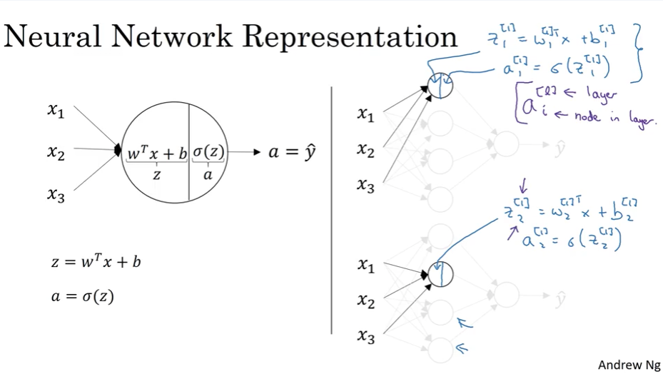
Step 1: Compute linear combination

\[z^{[1]}_1 = (w^{[1]}_1)^T x + b^{[1]}_1\]

Step 2: Apply activation function

\[a^{[1]}_1 = \sigma(z^{[1]}_1)\]

Notation reminder:

Superscript $[1]$: layer number (hidden layer)
Subscript $1$: node number (first node)

Second Hidden Unit (Node 2)

The second node follows the same pattern with different parameters:

\[z^{[1]}_2 = (w^{[1]}_2)^T x + b^{[1]}_2\] \[a^{[1]}_2 = \sigma(z^{[1]}_2)\]

All Four Hidden Units

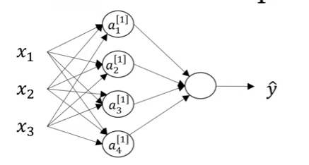
For a network with 4 hidden units, we have:

\[z^{[1]}_1 = (w^{[1]}_1)^T x + b^{[1]}_1, \quad a^{[1]}_1 = \sigma(z^{[1]}_1)\] \[z^{[1]}_2 = (w^{[1]}_2)^T x + b^{[1]}_2, \quad a^{[1]}_2 = \sigma(z^{[1]}_2)\] \[z^{[1]}_3 = (w^{[1]}_3)^T x + b^{[1]}_3, \quad a^{[1]}_3 = \sigma(z^{[1]}_3)\] \[z^{[1]}_4 = (w^{[1]}_4)^T x + b^{[1]}_4, \quad a^{[1]}_4 = \sigma(z^{[1]}_4)\]

Problem: Computing with a for-loop over each node is inefficient. Let’s vectorize!

Vectorizing the Hidden Layer

Instead of computing each node separately, we can process all nodes simultaneously using matrix operations.

Creating the Weight Matrix

Stack the weight vectors as rows in a matrix:

\[W^{[1]} = \begin{bmatrix} — (w^{[1]}_1)^T — \\ — (w^{[1]}_2)^T — \\ — (w^{[1]}_3)^T — \\ — (w^{[1]}_4)^T — \end{bmatrix}\]

This creates a $(4 \times 3)$ matrix where:

4 rows = 4 hidden units
3 columns = 3 input features

Matrix Multiplication

Now compute all $z$ values at once:

\[W^{[1]} \cdot x = \begin{bmatrix} (w^{[1]}_1)^T x \\ (w^{[1]}_2)^T x \\ (w^{[1]}_3)^T x \\ (w^{[1]}_4)^T x \end{bmatrix}\]

Adding Bias Vector

Stack biases vertically:

\[b^{[1]} = \begin{bmatrix} b^{[1]}_1 \\ b^{[1]}_2 \\ b^{[1]}_3 \\ b^{[1]}_4 \end{bmatrix}\]

Complete Hidden Layer Computation

Linear step:

\[z^{[1]} = W^{[1]} x + b^{[1]}\]

where $z^{[1]} = \begin{bmatrix} z^{[1]}_1 \ z^{[1]}_2 \ z^{[1]}_3 \ z^{[1]}_4 \end{bmatrix}$

Activation step:

\[a^{[1]} = \sigma(z^{[1]})\]

The sigmoid function is applied element-wise to the vector $z^{[1]}$.

Vectorization Rule of Thumb

Key principle: Different nodes in a layer are stacked vertically in column vectors.

Computing the Output Layer

The output layer follows the same pattern:

\[z^{[2]} = W^{[2]} a^{[1]} + b^{[2]}\] \[a^{[2]} = \sigma(z^{[2]})\]

where:

$W^{[2]}$: shape $(1 \times 4)$ - one output unit receiving from 4 hidden units
$b^{[2]}$: shape $(1 \times 1)$ - scalar bias
$a^{[1]}$: shape $(4 \times 1)$ - activations from hidden layer

The output $a^{[2]}$ is our prediction: $\hat{y} = a^{[2]}$

Insight: The output layer is just one logistic regression unit that takes the hidden layer activations as its input.

Complete Forward Propagation (Single Example)

Using Input Notation $x$

Hidden layer:

Z1 = np.dot(W1, x) + b1    # Shape: (4, 1) = (4, 3) @ (3, 1) + (4, 1)
A1 = sigmoid(Z1)            # Shape: (4, 1)

Output layer:

Z2 = np.dot(W2, A1) + b2   # Shape: (1, 1) = (1, 4) @ (4, 1) + (1, 1)
A2 = sigmoid(Z2)            # Shape: (1, 1)

Prediction:

y_hat = A2

Using Activation Notation $a^{[0]}$

Recall that $x = a^{[0]}$ (input layer activations). We can equivalently write:

\[z^{[1]} = W^{[1]} a^{[0]} + b^{[1]}\] \[a^{[1]} = \sigma(z^{[1]})\] \[z^{[2]} = W^{[2]} a^{[1]} + b^{[2]}\] \[a^{[2]} = \sigma(z^{[2]}) = \hat{y}\]

Dimension Analysis

Let’s verify the matrix dimensions work correctly:

Computation	Matrix Dimensions	Result
$W^{[1]} x$	$(4 \times 3) \cdot (3 \times 1)$	$(4 \times 1)$
$z^{[1]} = W^{[1]} x + b^{[1]}$	$(4 \times 1) + (4 \times 1)$	$(4 \times 1)$
$a^{[1]} = \sigma(z^{[1]})$	$\sigma((4 \times 1))$	$(4 \times 1)$
$W^{[2]} a^{[1]}$	$(1 \times 4) \cdot (4 \times 1)$	$(1 \times 1)$
$z^{[2]} = W^{[2]} a^{[1]} + b^{[2]}$	$(1 \times 1) + (1 \times 1)$	$(1 \times 1)$
$a^{[2]} = \sigma(z^{[2]})$	$\sigma((1 \times 1))$	$(1 \times 1)$

All dimensions are compatible! ✓

Comparison with Logistic Regression

Aspect	Logistic Regression	Neural Network
Computation	$z = w^T x + b$ $a = \sigma(z)$	Hidden: $z^{[1]} = W^{[1]} x + b^{[1]}, a^{[1]} = \sigma(z^{[1]})$ Output: $z^{[2]} = W^{[2]} a^{[1]} + b^{[2]}, a^{[2]} = \sigma(z^{[2]})$
Lines of code	2	4
Parameters	$w, b$	$W^{[1]}, b^{[1]}, W^{[2]}, b^{[2]}$
Layers	1 (output only)	2 (hidden + output)

Implementation Summary

To compute the output of a 2-layer neural network for a single example, you need just 4 lines:

# Hidden layer
Z1 = np.dot(W1, x) + b1
A1 = sigmoid(Z1)

# Output layer
Z2 = np.dot(W2, A1) + b2
A2 = sigmoid(Z2)

# Prediction
y_hat = A2

Key Takeaways

Each node performs two steps: linear combination ($z$) then activation ($a$)
A neural network is logistic regression repeated for each node in each layer
Vectorization eliminates for-loops by processing all nodes simultaneously
Stack weight vectors as rows in $W^{[l]}$ to enable matrix multiplication
Stack node outputs vertically in column vectors $z^{[l]}$ and $a^{[l]}$
Forward propagation for one example requires only 4 equations (or 4 lines of code)
Matrix dimensions must be compatible: $(n^{[l]} \times n^{[l-1]}) \cdot (n^{[l-1]} \times 1) = (n^{[l]} \times 1)$

Computing a Neural Network’s Output

Table of contents