Last modified: Jan 31 2026 at 10:09 PM • 6 mins read

Activation Functions

Table of contents

1. Introduction
2. What is an Activation Function?
3. Common Activation Functions
4. Comparison Table
5. Practical Guidelines
6. Choosing the Right Activation Function
7. Implementation Example
8. Key Takeaways

---

Introduction

When building a neural network, one of the key decisions you need to make is choosing the activation function for hidden layers and the output layer. So far, we’ve only used the sigmoid function, but several other options often work much better. Let’s explore the most common activation functions and learn when to use each one.

What is an Activation Function?

In forward propagation, we compute:

\[z^{[l]} = W^{[l]} a^{[l-1]} + b^{[l]}\] \[a^{[l]} = g^{[l]}(z^{[l]})\]

The function $g(z)$ is called the activation function. It introduces non-linearity into the network, allowing it to learn complex patterns.

Common Activation Functions

1. Sigmoid Function

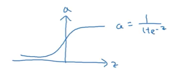
Formula:

\[\sigma(z) = \frac{1}{1 + e^{-z}}\]

Range: $(0, 1)$

Graph: S-shaped curve

Pros:

• Output is between 0 and 1
• Good for binary classification output layer
• Smooth gradient

Cons:

• ❌ Vanishing gradient problem (gradient near 0 for large/small $z$)
• ❌ Outputs not zero-centered (mean around 0.5)
• ❌ Slow convergence

When to use:

• ✅ Output layer for binary classification only
• ❌ Almost never use for hidden layers

2. Hyperbolic Tangent (tanh)

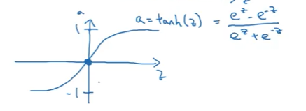
Formula:

\[\tanh(z) = \frac{e^z - e^{-z}}{e^z + e^{-z}}\]

Range: $(-1, 1)$

Graph: S-shaped curve, shifted version of sigmoid

Pros:

• Zero-centered (mean around 0)
• Better than sigmoid for hidden layers
• Data centering effect helps next layer learn faster

Cons:

• ❌ Still has vanishing gradient problem
• ❌ Computationally more expensive than ReLU

When to use:

• ✅ Hidden layers (better than sigmoid)
• ❌ Not recommended over ReLU in most cases

Why better than sigmoid?

By outputting values between -1 and 1 (instead of 0 and 1), tanh centers the data around zero. This makes learning easier for the next layer, similar to how normalizing input data helps training.

3. ReLU (Rectified Linear Unit)

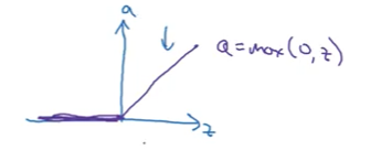
Formula:

\[\text{ReLU}(z) = \max(0, z) = \begin{cases} z & \text{if } z > 0 \\ 0 & \text{if } z \leq 0 \end{cases}\]

Range: $[0, \infty)$

Graph: Linear for positive values, zero for negative

Pros:

• ✅ No vanishing gradient for positive values
• ✅ Computationally efficient (simple max operation)
• ✅ Fast convergence in practice
• ✅ Most popular choice today

Cons:

• ❌ “Dying ReLU” - gradient is 0 when $z < 0$
• ❌ Not zero-centered

When to use:

• ✅ Default choice for hidden layers
• ✅ Use this if you’re unsure

Implementation note:

The derivative at $z = 0$ is technically undefined, but in practice, you can treat it as either 0 or 1 - it makes negligible difference since the probability of exactly hitting 0 is infinitesimally small.

4. Leaky ReLU

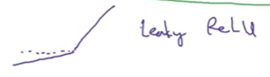
Formula:

\[\text{Leaky ReLU}(z) = \max(0.01z, z) = \begin{cases} z & \text{if } z > 0 \\ 0.01z & \text{if } z \leq 0 \end{cases}\]

Range: $(-\infty, \infty)$

Graph: Linear for positive, small slope (0.01) for negative

Pros:

• ✅ Fixes “dying ReLU” problem
• ✅ Never has zero gradient
• ✅ All benefits of ReLU plus gradient flow for negative values

Cons:

• Less commonly used than ReLU (but often performs better)

When to use:

• ✅ Alternative to ReLU
• ✅ Try if ReLU isn’t working well

Variations:

• The slope parameter (0.01) can be learned during training (called Parametric ReLU or PReLU)
• Some practitioners report better results, but it’s less common in practice

Comparison Table

Activation	Formula	Range	Hidden Layer	Output Layer	Pros	Cons
Sigmoid	$\frac{1}{1+e^{-z}}$	(0, 1)	❌ Avoid	✅ Binary classification	Smooth, probabilistic output	Vanishing gradient, not zero-centered
Tanh	$\frac{e^z-e^{-z}}{e^z+e^{-z}}$	(-1, 1)	⚠️ OK	❌ Rarely	Zero-centered	Vanishing gradient
ReLU	$\max(0, z)$	[0, ∞)	✅ Default	❌ No	Fast, efficient, no vanishing gradient	Dying ReLU problem
Leaky ReLU	$\max(0.01z, z)$	(-∞, ∞)	✅ Good	❌ No	Fixes dying ReLU	Less popular

Practical Guidelines

Rule of Thumb

1. Output Layer:
   • Binary classification → Sigmoid
   • Multi-class classification → Softmax (covered later)
   • Regression → Linear (no activation) or ReLU
2. Hidden Layers:
   • Default choice → ReLU
   • If ReLU doesn’t work well → Try Leaky ReLU
   • Rarely → tanh
   • Almost never → sigmoid

Why ReLU Works So Well

Despite having zero gradient for negative values, ReLU works because:

1. In practice, enough hidden units have $z > 0$
2. Learning remains fast for most training examples
3. The non-saturating gradient (gradient = 1 for $z > 0$) accelerates convergence

Layer-Specific Activation Functions

You can (and often should) use different activation functions for different layers:

Example for binary classification:

# Hidden layer 1
Z1 = np.dot(W1, X) + b1
A1 = relu(Z1)                    # ReLU

# Hidden layer 2  
Z2 = np.dot(W2, A1) + b2
A2 = relu(Z2)                    # ReLU

# Output layer
Z3 = np.dot(W3, A2) + b3
A3 = sigmoid(Z3)                 # Sigmoid for binary classification

Notation: Use superscripts to denote layer-specific functions: $g^{[1]}(z)$ vs $g^{[2]}(z)$

Choosing the Right Activation Function

The Pragmatic Approach

It’s often difficult to know in advance which activation function will work best for your specific problem. Best practice:

1. Start with ReLU as the default for hidden layers
2. Try multiple options: ReLU, Leaky ReLU, tanh
3. Evaluate on validation set to see which performs best
4. Iterate and experiment - no universal rule applies to all problems

Key insight: Deep learning involves many architectural choices (activation functions, number of units, initialization, etc.). Experimentation and empirical validation are essential parts of the process.

Future-Proofing Your Skills

Rather than memorizing “always use ReLU,” understand the trade-offs:

• What problems does each function solve?
• What are the computational costs?
• How do they affect gradient flow?

This knowledge helps you adapt to:

• New problem domains
• Evolving best practices
• Novel architectures

Implementation Example

import numpy as np

def sigmoid(z):
    """Sigmoid activation: (0, 1)"""
    return 1 / (1 + np.exp(-z))

def tanh(z):
    """Hyperbolic tangent: (-1, 1)"""
    return np.tanh(z)

def relu(z):
    """ReLU activation: [0, ∞)"""
    return np.maximum(0, z)

def leaky_relu(z, alpha=0.01):
    """Leaky ReLU activation: (-∞, ∞)"""
    return np.maximum(alpha * z, z)

# Example usage
z = np.array([-2, -1, 0, 1, 2])

print("Sigmoid:", sigmoid(z))
# [0.119, 0.268, 0.5, 0.731, 0.881]

print("Tanh:", tanh(z))
# [-0.964, -0.762, 0, 0.762, 0.964]

print("ReLU:", relu(z))
# [0, 0, 0, 1, 2]

print("Leaky ReLU:", leaky_relu(z))
# [-0.02, -0.01, 0, 1, 2]

Key Takeaways

1. Activation functions introduce non-linearity into neural networks
2. Sigmoid: Use only for binary classification output layer
3. Tanh: Better than sigmoid for hidden layers but still has vanishing gradient
4. ReLU: Default choice for hidden layers - fast, efficient, widely used
5. Leaky ReLU: Fixes dying ReLU problem, worth trying
6. Different layers can use different activations: ReLU for hidden, sigmoid for output
7. Vanishing gradient problem: Sigmoid and tanh suffer from this, ReLU doesn’t (for $z > 0$)
8. Experiment and validate: Try multiple activation functions on your validation set
9. No universal best choice: What works depends on your specific problem
10. Default recommendation: Start with ReLU for hidden layers