Last modified: Jan 31 2026 at 10:09 PM • 3 mins read
What is a Neural Network?
Table of contents
- Introduction
- Binary Classification Problem
- Image Representation in Computers
- Notation for Training Data
- Matrix Representation
- Key Convention
Introduction
This week covers essential neural network implementation techniques:
- Vectorization: Processing entire training sets without explicit for loops
- Forward and Backward Propagation: How computations are organized in neural networks
- Logistic Regression: Used as a foundation to understand these concepts
Binary Classification Problem
Logistic regression is an algorithm for binary classification. Let’s understand this through an example:
Example Task: Classify whether an image contains a cat or not
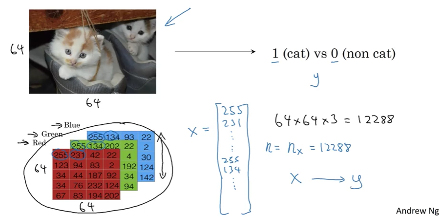
- Output:
y = 1(cat) ory = 0(not a cat)
Image Representation in Computers
RGB Color Channels
An image is stored as three separate matrices representing:
- Red channel
- Green channel
- Blue channel
For a 64×64 pixel image:
- Each channel: 64×64 matrix
- Total: 3 matrices of pixel intensity values
Converting Images to Feature Vectors
To use an image as input to a neural network, we unroll the pixel values into a feature vector $x$:
Process:
- List all red pixel values:
[255, 231, ..., ] - List all green pixel values:
[255, 134, ..., ] - List all blue pixel values:
[...] - Concatenate into one long vector
Dimension Calculation: \(n_x = 64 \times 64 \times 3 = 12,288\)
Where:
- $n_x$ = dimension of input feature vector
- Sometimes abbreviated as $n$
Goal: Learn a classifier that takes this feature vector $x$ and predicts label $y$ (1 or 0).
Notation for Training Data
Single Training Example
A single training example is a pair: $(x, y)$
- $x$: $n_x$-dimensional feature vector
- $y$: label (0 or 1)
Training Set Notation
Training set with $m$ examples: \((x^{(1)}, y^{(1)}), (x^{(2)}, y^{(2)}), \ldots, (x^{(m)}, y^{(m)})\)
Where:
- $m$ = number of training examples (sometimes written as $m_{train}$)
- $m_{test}$ = number of test examples
Matrix Representation
Input Matrix $X$
Stack all training examples as columns in a matrix:
\[X = [x^{(1)} \mid x^{(2)} \mid \cdots \mid x^{(m)}]\]Dimensions: $X$ is an $n_x \times m$ matrix
- Rows: $n_x$ (feature dimension)
- Columns: $m$ (number of examples)
Python notation: X.shape = (nx, m)
Why column-wise?
- Makes neural network implementation easier
- Different from some conventions that stack examples as rows
Output Matrix $Y$
Similarly, stack all labels as columns:
\[Y = [y^{(1)} \mid y^{(2)} \mid \cdots \mid y^{(m)}]\]Dimensions: $Y$ is a $1 \times m$ matrix
Python notation: Y.shape = (1, m)
Key Convention
Throughout this course:
- Data from different training examples are stacked in different columns
- Applies to inputs ($x$), outputs ($y$), and other quantities
- This convention simplifies neural network implementation