Last modified: Jan 31 2026 at 10:09 PM • 4 mins read
Gradient Descent
Table of contents
- Introduction
- Recap: Logistic Regression Setup
- Computation Graph (Forward Pass)
- Backward Propagation (Computing Derivatives)
- Summary of Derivatives for One Example
- Gradient Descent Update (One Example)
- Generalizing to $n$ Features
- The Big Picture
- What About Multiple Training Examples?
- Key Takeaways
Introduction
In this lesson, we’ll learn how to compute derivatives to implement gradient descent for logistic regression.
Goal: Understand the key equations needed to implement gradient descent.
Method: We’ll use a computation graph to visualize the process. While this might seem like overkill for logistic regression, it’s excellent preparation for understanding neural networks.
Recap: Logistic Regression Setup
For a single training example:
Prediction: \(\hat{y} = a = \sigma(z)\)
where: \(z = w^T x + b\)
Loss function: \(\mathcal{L}(a, y) = -[y \log(a) + (1-y) \log(1-a)]\)
Where:
- $a$ = output of logistic regression (same as $\hat{y}$)
- $y$ = true label
Objective: Modify parameters $w$ and $b$ to reduce the loss.
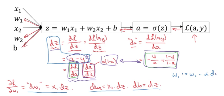
Computation Graph (Forward Pass)
Let’s visualize this for a simple example with 2 features: $x_1$ and $x_2$.
Inputs:
- Features: $x_1$, $x_2$
- Parameters: $w_1$, $w_2$, $b$
Forward computation steps:
Step 1: z = w₁x₁ + w₂x₂ + b
        ↓
Step 2: a = σ(z)
        ↓
Step 3: L(a,y) = loss
This is called forward propagation - computing from inputs to loss.
Backward Propagation (Computing Derivatives)
Now we go backwards through the computation graph to compute derivatives.
Step 1: Derivative with respect to $a$
Compute: $\frac{d\mathcal{L}}{da}$ (code variable: da)
Note: If you don’t know calculus, that’s okay! We provide all derivative formulas you need.
Step 2: Derivative with respect to $z$
Compute: $\frac{d\mathcal{L}}{dz}$ (code variable: dz)
For calculus experts: This uses the chain rule:
\[\frac{d\mathcal{L}}{dz} = \frac{d\mathcal{L}}{da} \cdot \frac{da}{dz}\]Where:
- $\frac{da}{dz} = a(1-a)$ (derivative of sigmoid)
- Multiplying these gives: $a - y$
Key insight: The derivative simplifies beautifully to just $a - y$!
Step 3: Derivatives with respect to parameters
Compute: $\frac{d\mathcal{L}}{dw_1}$, $\frac{d\mathcal{L}}{dw_2}$, $\frac{d\mathcal{L}}{db}$
\[\frac{d\mathcal{L}}{dw_1} = x_1 \cdot dz\] \[\frac{d\mathcal{L}}{dw_2} = x_2 \cdot dz\] \[\frac{d\mathcal{L}}{db} = dz\]Code variables: dw1, dw2, db
Summary of Derivatives for One Example
| Variable | Derivative Formula | Code Variable |
|---|---|---|
| $a$ | $-\frac{y}{a} + \frac{1-y}{1-a}$ | da |
| $z$ | $a - y$ | dz |
| $w_1$ | $x_1 \cdot (a - y)$ | dw1 |
| $w_2$ | $x_2 \cdot (a - y)$ | dw2 |
| $b$ | $a - y$ | db |
Gradient Descent Update (One Example)
Step 1: Compute derivatives
# Forward pass (already done)
z = w1*x1 + w2*x2 + b
a = sigmoid(z)
loss = -(y*log(a) + (1-y)*log(1-a))

# Backward pass
dz = a - y
dw1 = x1 * dz
dw2 = x2 * dz
db = dz
Step 2: Update parameters
w1 = w1 - alpha * dw1
w2 = w2 - alpha * dw2
b = b - alpha * db
Where $\alpha$ is the learning rate.
Generalizing to $n$ Features
For $n$ features $(x_1, x_2, \ldots, x_n)$:
\[z = \sum_{i=1}^{n} w_i x_i + b = w^T x + b\]Derivatives:
\[\frac{d\mathcal{L}}{dw_i} = x_i \cdot dz = x_i \cdot (a - y)\]In vectorized form:
\[\frac{d\mathcal{L}}{dw} = x \cdot dz\]The Big Picture
Forward propagation (compute loss):
x → z → a → L
Backward propagation (compute gradients):
x ← dz ← da ← dL
Update parameters:
w = w - α · dw
b = b - α · db
What About Multiple Training Examples?
So far, we’ve shown gradient descent for one training example. But in practice, we have $m$ training examples.
Next step: Learn how to apply these concepts to an entire training set efficiently.
Key Takeaways
- Forward propagation: Compute predictions and loss
- Backward propagation: Compute derivatives using the chain rule
- Key formula: $dz = a - y$ (prediction error)
- Update rule: Subtract learning rate times gradient
- Computation graph: Visual tool for understanding derivatives
Don’t worry about calculus: We provide all the derivative formulas you need. Focus on understanding the flow and implementing the updates correctly.