Last modified: Jan 31 2026 at 10:09 PM • 2 mins read
Logistic Regression
Table of contents
- Introduction
- Model Parameters
- Why Not Use Linear Regression?
- The Sigmoid Function
- Learning Objective
- Next Steps
Introduction
Logistic regression is a learning algorithm for binary classification problems where output labels $y$ are either 0 or 1.
Goal: Given an input feature vector $x$ (e.g., an image), output a prediction $\hat{y}$ that estimates $y$.
Formal Definition: \(\hat{y} = P(y=1 \mid x)\)
This represents the probability that $y = 1$ given the input features $x$.
Example: For a cat image classifier, $\hat{y}$ tells us the probability that the image contains a cat.
Model Parameters
Logistic regression has two sets of parameters:
- $w$: an $n_x$-dimensional weight vector
- $b$: a real number (bias term)
Question: Given input $x$ and parameters $w$ and $b$, how do we generate the output $\hat{y}$?
Why Not Use Linear Regression?
Linear Approach (Doesn’t Work)
You might try: \(\hat{y} = w^T x + b\)
Problem with this approach:
- $\hat{y}$ should be a probability between 0 and 1
- $w^T x + b$ can be any real number (greater than 1 or even negative)
- Negative probabilities don’t make sense
This is why linear regression isn’t suitable for binary classification.
The Sigmoid Function
Instead, logistic regression uses the sigmoid function to ensure output is between 0 and 1:
\[\hat{y} = \sigma(w^T x + b)\]Where: \(z = w^T x + b\)
Sigmoid Formula
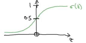
\[\sigma(z) = \frac{1}{1 + e^{-z}}\]Sigmoid Properties
Visual behavior:
- Smoothly increases from 0 to 1
- Crosses 0.5 at $z = 0$
- S-shaped curve
Mathematical analysis:
When $z$ is very large (positive):
- $e^{-z} \approx 0$
- $\sigma(z) \approx \frac{1}{1 + 0} = 1$
When $z$ is very small (large negative):
- $e^{-z}$ becomes very large
- $\sigma(z) \approx \frac{1}{1 + \text{huge number}} \approx 0$
Learning Objective
Your job when implementing logistic regression is to:
Learn parameters $w$ and $b$ such that $\hat{y}$ becomes a good estimate of the probability that $y = 1$.
Next Steps
Now that you understand the logistic regression model, the next step is to define a cost function to learn parameters $w$ and $b$.