Last modified: Jan 31 2026 at 10:09 PM • 4 mins read

Gradient Descent

Table of contents

1. Introduction
2. Visualizing Gradient Descent
3. How Gradient Descent Works
4. Understanding the Derivative
5. Full Gradient Descent for Logistic Regression
6. Understanding Notation: $d$ vs $\partial$
7. Implementation Summary
8. Key Takeaways

---

Introduction

Now that we have defined the cost function $J(w, b)$, we need an algorithm to minimize it and learn the optimal parameters $w$ and $b$. This algorithm is called gradient descent.

Recap:

\[J(w, b) = -\frac{1}{m} \sum_{i=1}^{m} \left[y^{(i)} \log(\hat{y}^{(i)}) + (1-y^{(i)}) \log(1-\hat{y}^{(i)})\right]\]

Goal: Find $w$ and $b$ that minimize $J(w, b)$.

Visualizing Gradient Descent

The Cost Function Surface

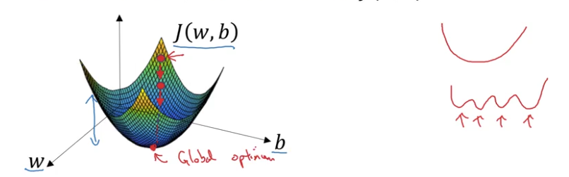
Imagine the cost function as a 3D surface:

• Horizontal axes: Parameters $w$ and $b$
  • (In practice, $w$ can be high-dimensional, but we’ll use 1D for visualization)
• Vertical axis: Value of $J(w, b)$
• Surface height: The cost at each point

Convex vs Non-Convex Functions

Convex function (our logistic regression cost):

• Single “bowl” shape
• One global minimum
• No local minima

Non-convex function:

• Multiple “hills and valleys”
• Many local minima
• Harder to optimize

Why this matters: Our cost function $J(w, b)$ is convex, which is why we chose this particular function. This guarantees we can find the global minimum.

How Gradient Descent Works

The Algorithm

Step 1: Initialize

• Start with initial values for $w$ and $b$ (usually $w = 0$, $b = 0$)
• Because the function is convex, initialization doesn’t matter much

Step 2: Repeat until convergence

• Take a step in the steepest downhill direction
• Move toward lower cost
• Each step brings us closer to the minimum

Step 3: Converge

• Eventually reach the global minimum (or very close to it)

Mathematical Update Rule

For a simplified 1D case (just parameter $w$):

\[w := w - \alpha \frac{dJ(w)}{dw}\]

Where:

• $:=$ means “update” or “assign”
• $\alpha$ is the learning rate (controls step size)
• $\frac{dJ(w)}{dw}$ is the derivative (slope of the cost function)

Code convention: We use dw as the variable name for $\frac{dJ(w)}{dw}$

w = w - alpha * dw

Understanding the Derivative

What is a Derivative?

The derivative $\frac{dJ(w)}{dw}$ represents the slope of the cost function at the current point.

Intuition:

• Slope = height / width of the tangent line
• Tells us which direction is “downhill”
• Tells us how steep the slope is

How the Update Works

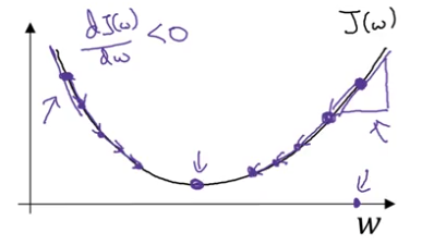
Case 1: Positive slope (derivative > 0)

• If $w$ is to the right of the minimum
• Derivative is positive
• $w := w - \alpha \times (\text{positive}) = w - \text{positive}$
• $w$ decreases → moves left toward minimum

Case 2: Negative slope (derivative < 0)

• If $w$ is to the left of the minimum
• Derivative is negative
• $w := w - \alpha \times (\text{negative}) = w + \text{positive}$
• $w$ increases → moves right toward minimum

Result: Regardless of where you start, gradient descent moves you toward the minimum.

Full Gradient Descent for Logistic Regression

For logistic regression with parameters $w$ and $b$:

Update rules:

\[w := w - \alpha \frac{\partial J(w,b)}{\partial w}\] \[b := b - \alpha \frac{\partial J(w,b)}{\partial b}\]

Code convention:

w = w - alpha * dw  # dw represents ∂J/∂w
b = b - alpha * db  # db represents ∂J/∂b

Understanding Notation: $d$ vs $\partial$

The Confusing Calculus Notation

Single variable (one parameter):

• Use regular $d$: $\frac{dJ(w)}{dw}$

Multiple variables (two or more parameters):

• Use partial derivative $\partial$: $\frac{\partial J(w,b)}{\partial w}$

Important: They mean almost the same thing! Both represent the slope with respect to one variable.

Why This Notation Exists

The rule is:

• $J(w)$ → use $\frac{d}{dw}$ (ordinary derivative)
• $J(w, b)$ → use $\frac{\partial}{\partial w}$ (partial derivative)

Don’t worry too much about this distinction - both measure the slope in one direction.

Implementation Summary

In code, we use these conventions:

Mathematical Notation	Code Variable	Meaning
$\frac{\partial J(w,b)}{\partial w}$	dw	Amount to update $w$
$\frac{\partial J(w,b)}{\partial b}$	db	Amount to update $b$
$\alpha$	alpha or learning_rate	Step size

Update step:

# Compute gradients (we'll learn how in next lessons)
dw = compute_gradient_w(...)
db = compute_gradient_b(...)

# Update parameters
w = w - alpha * dw
b = b - alpha * db

Key Takeaways

1. Gradient descent finds the minimum of the cost function
2. The derivative (slope) tells us which direction to move
3. The learning rate $\alpha$ controls how big each step is
4. We repeat the update until convergence
5. Because $J(w,b)$ is convex, we always reach the global minimum