Last modified: Jan 31 2026 at 10:09 PM • 3 mins read
Why Regularization Reduces Overfitting?
Table of contents
- Introduction
- Problem: Understanding Regularization’s Effect
- Intuition 1: Network Simplification Through Weight Reduction
- Intuition 2: Linear Activation Regime
- Implementation Considerations
- Key Takeaways
Introduction
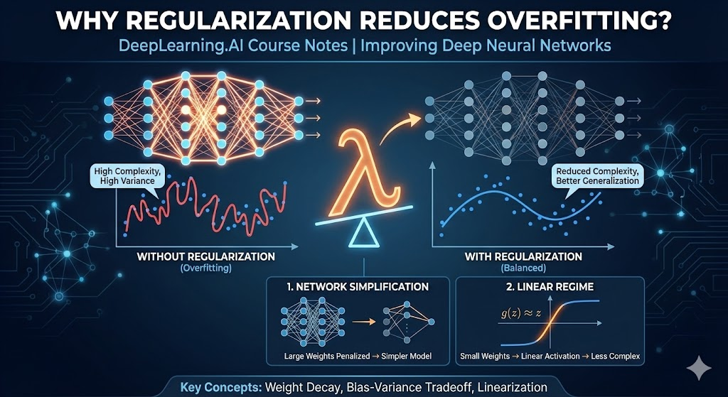
Regularization is a crucial technique for preventing overfitting in neural networks. This lesson explores the intuitive reasons why regularization works and provides two key perspectives on how it reduces model complexity.
Problem: Understanding Regularization’s Effect
When we add regularization to our cost function, we modify it from:
\[J(W,b) = \frac{1}{m} \sum_{i=1}^{m} \mathcal{L}(y^{(i)}, \hat{y}^{(i)})\]to:
\[J(W,b) = \frac{1}{m} \sum_{i=1}^{m} \mathcal{L}(y^{(i)}, \hat{y}^{(i)}) + \frac{\lambda}{2m} \sum_{l=1}^{L} \|W^{[l]}\|_F^2\]The question is: Why does penalizing large weights reduce overfitting?
Intuition 1: Network Simplification Through Weight Reduction
The Mechanism
When we set the regularization parameter $\lambda$ to be very large:
- Weight Penalization: The cost function heavily penalizes large weights
- Weight Shrinkage: Weights $W^{[l]}$ are driven toward zero
- Hidden Unit Impact: Many hidden units have greatly reduced influence
- Effective Simplification: The network behaves like a much smaller, simpler model
Mathematical Perspective
For large $\lambda$:
- Weights approach zero: $W^{[l]} \to 0$
- Hidden unit activations become negligible
- Complex network → Simple linear-like model
Bias-Variance Trade-off
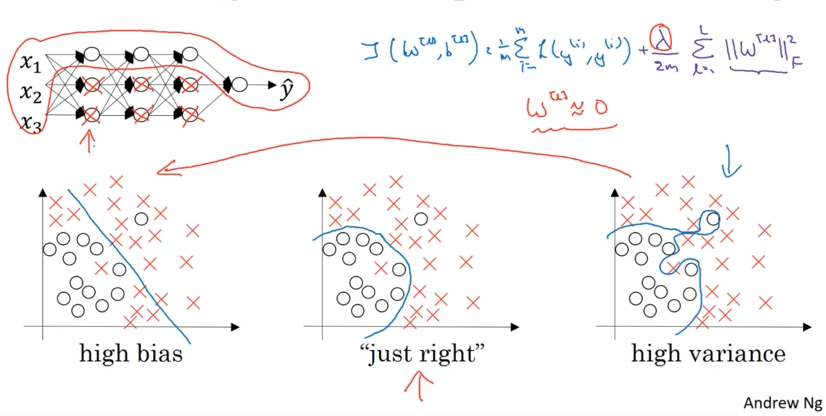
| Regularization Level | Network Complexity | Bias | Variance | Result |
|---|---|---|---|---|
| $\lambda = 0$ | High complexity | Low | High | Overfitting |
| $\lambda$ very large | Low complexity | High | Low | Underfitting |
| $\lambda$ optimal | Moderate complexity | Moderate | Moderate | Good fit |
Important Clarification
Note: In practice, regularization doesn’t completely zero out hidden units. Instead, it reduces their individual impact while keeping all units active, resulting in a smoother, less complex function.
Intuition 2: Linear Activation Regime
Activation Function Analysis
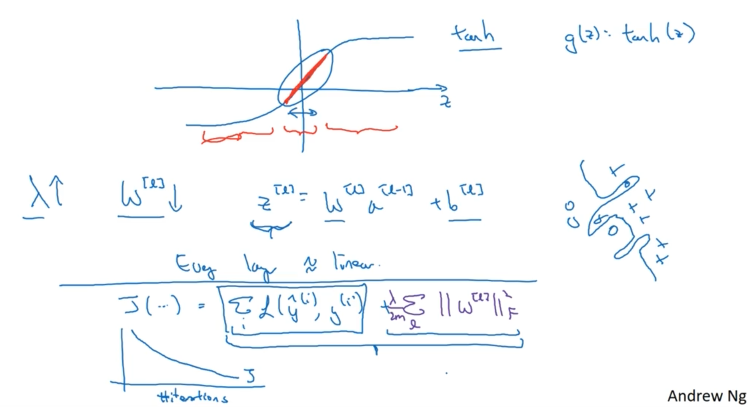
Consider the $\tanh$ activation function:
\[g(z) = \tanh(z)\]Key observation: When $z$ is small, $\tanh(z) \approx z$ (linear regime)
How Regularization Creates Linearity
- Weight Reduction: Large $\lambda$ → Small weights $W^{[l]}$
- Small Linear Combinations: $z^{[l]} = W^{[l]}a^{[l-1]} + b^{[l]}$ becomes small
- Linear Activation: When $|z^{[l]}|$ is small, $g(z^{[l]}) \approx z^{[l]}$
- Network Linearization: Each layer becomes approximately linear
Mathematical Chain
\[\text{Large } \lambda \to \text{Small } W^{[l]} \to \text{Small } z^{[l]} \to \text{Linear } g(z^{[l]}) \to \text{Linear Network}\]Why Linear Networks Can’t Overfit
- Limited Expressiveness: Linear functions can only create linear decision boundaries
- Reduced Capacity: Cannot fit complex, highly non-linear patterns
- Overfitting Prevention: Unable to memorize training data noise
Implementation Considerations
Debugging Gradient Descent with Regularization
When implementing regularization, remember to monitor the complete cost function:
# Correct: Include regularization term
J_total = J_loss + (lambda_reg / (2 * m)) * regularization_term

# Monitor J_total for monotonic decrease
plt.plot(iterations, J_total_history)
Warning: If you only plot the original loss term $J_{loss}$, you might not see monotonic decrease during training.
Cost Function Components
| Component | Formula | Purpose |
|---|---|---|
| Loss Term | $\frac{1}{m} \sum_{i=1}^{m} \mathcal{L}(y^{(i)}, \hat{y}^{(i)})$ | Fit training data |
| Regularization Term | $\frac{\lambda}{2m} \sum_{l=1}^{L} |W^{[l]}|_F^2$ | Prevent overfitting |
| Total Cost | Loss + Regularization | Balance fit and complexity |
Key Takeaways
- Weight Shrinkage: Regularization reduces weight magnitudes, simplifying the network
- Activation Linearization: Small weights keep activations in linear regime, reducing complexity
- Bias-Variance Balance: Proper $\lambda$ selection balances underfitting and overfitting
- Implementation: Always monitor the complete regularized cost function during training
- Practical Impact: L2 regularization is one of the most commonly used techniques in deep learning