Last modified: Jan 31 2026 at 10:09 PM • 6 mins read
Other Regularization Methods
Table of contents
Introduction
Beyond L2 regularization and dropout, there are additional techniques to reduce overfitting in neural networks. This lesson covers two important methods: data augmentation and early stopping.
Data Augmentation
The Problem: Not Enough Training Data
Ideal Solution: Collect more training data
Reality: Getting more data is often:
- Expensive (requires labeling, collection efforts)
- Time-consuming
- Sometimes impossible
Practical Solution: Augment your existing training data by creating modified versions of your examples.
Augmentation Techniques for Images
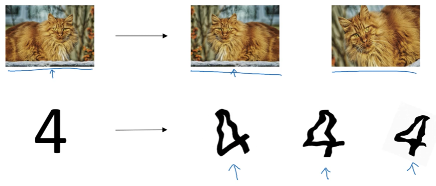
1. Horizontal Flipping
Technique: Mirror the image horizontally
Example - Cat Classifier:
import numpy as np
from PIL import Image

# Original image
original_cat = Image.open('cat.jpg')

# Flip horizontally
flipped_cat = original_cat.transpose(Image.FLIP_LEFT_RIGHT)

# Now you have 2 training examples instead of 1
Result: Double your training set size with minimal effort
Trade-off: The augmented examples are not as valuable as completely independent new examples, but they’re essentially free (except for computational cost).
Important: Notice we flip horizontally but NOT vertically—upside-down cats aren’t realistic examples!
2. Random Crops and Zooms
Technique: Take random sections of the image at different scales
import random

def random_crop(image, crop_size):
    """Randomly crop a portion of the image"""
    width, height = image.size
    left = random.randint(0, width - crop_size)
    top = random.randint(0, height - crop_size)

    return image.crop((left, top, left + crop_size, top + crop_size))

# Create multiple crops from one image
crops = [random_crop(original_cat, 224) for _ in range(5)]
Why It Works: A zoomed-in portion of a cat is still a cat—you’re teaching the model that the object can appear at different positions and scales.
3. Rotations and Distortions
Applications: Particularly useful for optical character recognition (OCR)
Example - Digit Recognition:
from scipy.ndimage import rotate

# Original digit "4"
digit = load_digit_image('four.png')

# Apply subtle rotation
rotated_digit = rotate(digit, angle=15, reshape=False)

# Apply distortion (elastic deformation)
distorted_digit = apply_elastic_distortion(digit)
Note on Distortion Strength:
- For demonstration: Strong distortions make the concept clear
- In practice: Use subtle distortions—you don’t want extremely warped digits that look unnatural
What Data Augmentation Teaches Your Model
By synthesizing augmented examples, you’re explicitly telling your algorithm:
| Transformation | Invariance Learned |
|---|---|
| Horizontal flip | “A cat facing left is still a cat” |
| Random crop/zoom | “A cat at different scales/positions is still a cat” |
| Rotation | “A slightly tilted digit is still the same digit” |
| Distortion | “Handwriting variations don’t change the digit identity” |
Data Augmentation as Regularization
How It Regularizes:
- Increases effective training set size → More data to learn from
- Introduces controlled variation → Prevents memorization of exact pixel patterns
- Low cost → Almost free regularization (just computation)
Comparison:
| Method | Cost | Data Increase | Independence |
|---|---|---|---|
| Collect new data | High | 100% | Fully independent |
| Data augmentation | Low | Variable | Somewhat redundant |
Early Stopping
The Concept
Idea: Stop training your neural network before it fully converges on the training set.
How It Works
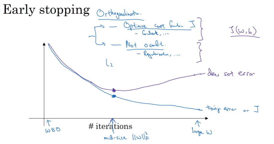
Step 1: Track Two Metrics During Training
Plot both metrics as training progresses:
- Training error (or cost function $J$) → Should decrease monotonically
- Dev set error → Initially decreases, then starts increasing
Step 2: Identify the Optimal Point
Typical Behavior:
\[\text{Iteration} \rightarrow \begin{cases} J_{\text{train}} & \searrow \text{(keeps decreasing)} \\ J_{\text{dev}} & \searrow \text{then} \nearrow \text{(starts increasing)} \end{cases}\]Decision: Stop training at the iteration where dev set error is lowest.
# Pseudocode for early stopping
best_dev_error = float('inf')
patience = 10
wait = 0

for iteration in range(max_iterations):
    train_one_epoch()

    dev_error = evaluate_on_dev_set()

    if dev_error < best_dev_error:
        best_dev_error = dev_error
        save_model()
        wait = 0
    else:
        wait += 1

    if wait >= patience:
        print(f"Early stopping at iteration {iteration}")
        break
Why Early Stopping Works
Connection to Weight Magnitudes:
- Early in training: Random initialization → Weights $w$ are small
- As training progresses: Weights grow larger and larger
- Early stopping effect: Stops training while weights are still mid-sized
Result: Smaller weight norms → Less overfitting
The Downside: Orthogonalization Violation
The Principle of Orthogonalization
Ideal Machine Learning Workflow: Separate concerns into independent tasks
| Task | Goal | Tools |
|---|---|---|
| 1. Optimize cost function | Minimize $J(w,b)$ | Gradient descent, Adam, RMSprop |
| 2. Prevent overfitting | Reduce variance | L2 regularization, dropout, more data |
Orthogonalization: Work on one task at a time with dedicated tools for each task.
Note: Adam (Adaptive Moment Estimation) and RMSprop (Root Mean Square Propagation) are advanced optimization algorithms that improve upon basic gradient descent. They adaptively adjust learning rates for each parameter, leading to faster and more stable convergence.
Why Early Stopping Violates This Principle
The Problem: Early stopping couples both tasks together
- Task 1 Impact: You stop optimizing $J$ before it’s fully minimized → Not doing a great job at Task 1
- Task 2 Impact: You’re simultaneously trying to prevent overfitting → Mixed objective
Consequence: The search space becomes more complicated—you can’t independently tune optimization and regularization.
Early Stopping vs L2 Regularization
Alternative Approach: Use L2 Regularization Instead
# Train as long as possible with L2 regularization
for lambda_val in [0.001, 0.01, 0.1, 1.0]:
    model = train_with_L2_regularization(lambda_val)
    evaluate(model)
Comparison:
| Aspect | Early Stopping | L2 Regularization |
|---|---|---|
| Orthogonalization | Violates (couples tasks) | Maintains (separate tasks) |
| Hyperparameter Search | Single training run explores multiple $|w|$ | Must try multiple $\lambda$ values |
| Computational Cost | Lower (one training run) | Higher (multiple training runs) |
| Search Space | More complex | Easier to decompose |
| Preference | Andrew Ng: Less preferred | Andrew Ng: Preferred (if affordable) |
When to Use Each
Use Early Stopping When:
- Computational budget is limited
- You want quick experimentation
- Training is very expensive
Use L2 Regularization When:
- You can afford multiple training runs
- You want cleaner separation of concerns
- You have the resources to search over $\lambda$
Early Stopping Benefits
Despite its downside, early stopping offers a unique advantage:
Key Benefit: In a single gradient descent run, you automatically try out small, medium, and large weight values without explicitly searching over the regularization hyperparameter $\lambda$.
Summary Comparison
| Technique | How It Works | Pros | Cons | Use Case |
|---|---|---|---|---|
| Data Augmentation | Create synthetic training examples through transformations | Nearly free, increases data | Less valuable than real data | Almost always beneficial |
| Early Stopping | Stop training when dev error increases | Low computational cost | Couples optimization and regularization | Limited compute budget |
| L2 Regularization | Penalize large weights with $\lambda$ | Clean separation of concerns | Requires multiple training runs | When you can afford it |
Key Takeaways
- Data augmentation is an inexpensive way to increase your effective training set size
- Common augmentations:
- Horizontal flipping (but usually not vertical)
- Random crops and zooms
- Rotations and subtle distortions
- Early stopping prevents overfitting by halting training when dev error starts increasing
- Early stopping works by keeping weight magnitudes small (similar to L2 regularization)
- Orthogonalization principle: Ideally, separate optimization and regularization into independent tasks
- Early stopping violates orthogonalization by coupling both tasks
- Preferred approach: L2 regularization (if computationally affordable) for cleaner hyperparameter search
- Practical choice: Early stopping is still widely used when compute is limited