Last modified: Jan 31 2026 at 10:09 PM • 6 mins read

Normalizing Inputs

Table of contents

1. Introduction
2. The Two-Step Normalization Process
3. Critical Rule: Use Training Statistics for Test Set
4. Why Normalization Speeds Up Training
5. When to Normalize: Practical Guidelines
6. Complete Workflow Example
7. Key Takeaways

---

Introduction

Normalizing your inputs is one of the most effective techniques to speed up neural network training. This preprocessing step ensures all input features are on similar scales, making optimization much more efficient.

The Two-Step Normalization Process

Consider a training set with input features $x$ (for example, 2-dimensional features visualized in a scatter plot).

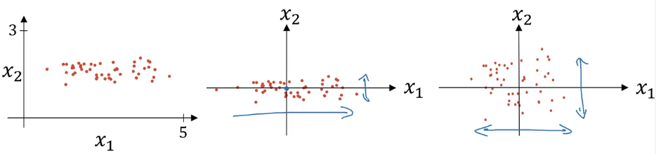
Step 1: Zero Out the Mean (Centering)

Goal: Shift all data so it’s centered around the origin

Formula:

\[\mu = \frac{1}{m} \sum_{i=1}^{m} x^{(i)}\] \[x := x - \mu\]

Where:

• $\mu$ is a vector containing the mean of each feature
• $m$ is the number of training examples
• $x^{(i)}$ is the $i$-th training example

Effect: This moves the entire training set so it has zero mean.

import numpy as np

# Calculate mean
mu = np.mean(X_train, axis=0)  # Shape: (n_features,)

# Subtract mean from all examples
X_train_centered = X_train - mu

Step 2: Normalize the Variances (Scaling)

Goal: Scale features so they have similar ranges

Formula:

\[\sigma^2 = \frac{1}{m} \sum_{i=1}^{m} (x^{(i)})^2\] \[x := \frac{x}{\sigma}\]

Where:

• $\sigma^2$ is a vector containing the variance of each feature (element-wise)
• $(x^{(i)})^2$ represents element-wise squaring
• Since we already subtracted the mean, this directly gives us the variance

Effect: Features $x_1$ and $x_2$ now both have variance equal to 1.

# Calculate standard deviation (after centering)
sigma = np.std(X_train_centered, axis=0)  # Shape: (n_features,)

# Normalize by standard deviation
X_train_normalized = X_train_centered / sigma

Complete Implementation:

def normalize_inputs(X_train, X_test):
    """
    Normalize training and test sets
    
    Args:
        X_train: Training data (m_train, n_features)
        X_test: Test data (m_test, n_features)
    
    Returns:
        X_train_norm, X_test_norm: Normalized datasets
    """
    # Step 1: Calculate mean and std from TRAINING data only
    mu = np.mean(X_train, axis=0)
    sigma = np.std(X_train, axis=0)
    
    # Step 2: Apply same transformation to both train and test
    X_train_norm = (X_train - mu) / sigma
    X_test_norm = (X_test - mu) / sigma
    
    return X_train_norm, X_test_norm

Critical Rule: Use Training Statistics for Test Set

Important: Always use the same $\mu$ and $\sigma$ (calculated from training data) to normalize both training and test sets.

Why?

• Training and test data must go through identical transformations
• If you calculate separate statistics for test data, you’re applying a different transformation
• This violates the assumption that train and test come from the same distribution

Correct Approach:

Step	Training Set	Test Set
Calculate $\mu$ and $\sigma$	✅ From training data	❌ Don’t calculate separately
Apply normalization	Use training $\mu$ and $\sigma$	Use same training $\mu$ and $\sigma$

Why Normalization Speeds Up Training

The Problem: Elongated Cost Functions

When features are on very different scales, the cost function becomes distorted:

Example - Unnormalized Features:

• Feature $x_1$: ranges from 1 to 1,000
• Feature $x_2$: ranges from 0 to 1

Impact on Cost Function $J(w, b)$:

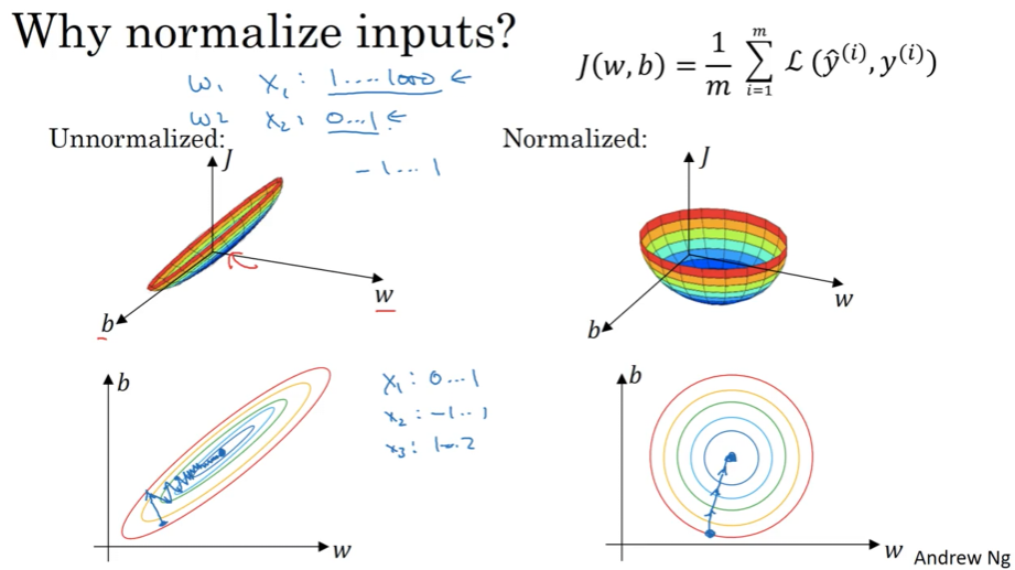
The contours become extremely elongated (like a stretched ellipse), because:

• Parameters $w_1$ and $w_2$ must compensate for vastly different input scales
• The cost function is much more sensitive to changes in $w_1$ than $w_2$
• Creates a “narrow valley” in the optimization landscape

The Solution: Spherical Cost Functions

After Normalization:

• All features roughly range from -1 to 1
• Features have similar variances (typically 1)

Result: Cost function contours become more spherical (circular) and symmetric.

Impact on Gradient Descent

Aspect	Unnormalized Features	Normalized Features
Cost Function Shape	Elongated ellipse	Spherical/circular
Learning Rate	Must use very small rate	Can use larger rate
Convergence Path	Oscillates back and forth	Direct path to minimum
Number of Steps	Many iterations needed	Fewer iterations
Training Speed	Slow	Fast

High-Dimensional Intuition

Note: In practice, $w$ is high-dimensional, so we can’t perfectly visualize this in 2D. But the key intuition holds: normalized features create a more round, easier-to-optimize cost function.

When to Normalize: Practical Guidelines

Always Normalize When

Features are on dramatically different scales

Examples:

Scenario	Feature 1 Range	Feature 2 Range	Normalize?
Housing prices	$100,000 - $1,000,000	1 - 5 bedrooms	✅ Critical
Medical data	Age: 0-100	White blood cells: 0-10,000	✅ Critical
Images (pixels)	Already 0-255	Already 0-255	✅ Still recommended (0-1)

Optional When

Features are already on similar scales

Examples:

Feature 1	Feature 2	Feature 3	Normalize?
0 to 1	-1 to 1	1 to 2	Optional (but harmless)
-0.5 to 0.5	-0.3 to 0.7	-0.2 to 0.8	Optional (but harmless)

Rule of Thumb:

• ✅ Critical when features differ by orders of magnitude (e.g., 1-1000 vs 0-1)
• ⚠️ Helpful when features differ by a factor of 10+
• ✔️ Optional but harmless when features are already similar

Best Practice: When in doubt, normalize anyway—it never hurts and often helps!

Complete Workflow Example

import numpy as np
import matplotlib.pyplot as plt

# Sample dataset with different scales
np.random.seed(42)
X_train = np.random.randn(100, 2)
X_train[:, 0] = X_train[:, 0] * 500 + 5000  # Feature 1: 4000-6000 range
X_train[:, 1] = X_train[:, 1] * 2           # Feature 2: -4 to 4 range

X_test = np.random.randn(20, 2)
X_test[:, 0] = X_test[:, 0] * 500 + 5000
X_test[:, 1] = X_test[:, 1] * 2

print("Before normalization:")
print(f"Feature 1 - Mean: {X_train[:, 0].mean():.1f}, Std: {X_train[:, 0].std():.1f}")
print(f"Feature 2 - Mean: {X_train[:, 1].mean():.1f}, Std: {X_train[:, 1].std():.1f}")

# Normalize using training statistics
mu = np.mean(X_train, axis=0)
sigma = np.std(X_train, axis=0)

X_train_norm = (X_train - mu) / sigma
X_test_norm = (X_test - mu) / sigma  # Use SAME mu and sigma!

print("\nAfter normalization:")
print(f"Feature 1 - Mean: {X_train_norm[:, 0].mean():.2f}, Std: {X_train_norm[:, 0].std():.2f}")
print(f"Feature 2 - Mean: {X_train_norm[:, 1].mean():.2f}, Std: {X_train_norm[:, 1].std():.2f}")

Output:

Before normalization:
Feature 1 - Mean: 5001.2, Std: 494.3
Feature 2 - Mean: 0.1, Std: 1.9

After normalization:
Feature 1 - Mean: 0.00, Std: 1.00
Feature 2 - Mean: 0.00, Std: 1.00

Key Takeaways

1. Two-step process:
   • First, subtract the mean ($x := x - \mu$)
   • Then, divide by standard deviation ($x := x / \sigma$)

2. Critical rule: Use training set statistics ($\mu$, $\sigma$) for both training and test sets

3. Why it works:
   • Unnormalized features → elongated cost function → slow, oscillating gradient descent
   • Normalized features → spherical cost function → fast, direct convergence
4. When to use:
   • Always when features have dramatically different scales (orders of magnitude)
   • Recommended as standard practice—it never hurts
   • Optional when features already have similar scales

5. Impact: Can dramatically speed up training by allowing larger learning rates and more direct optimization paths

6. Implementation tip: Always normalize before training, and save $\mu$ and $\sigma$ to apply the same transformation at inference time